Week 6 - CHT Analysis on a Graphics card
CONJUGATE HEAT TRANSFER ANALYSIS ON A GRAPHICS CARD
AIM:
To Perform Conjugate Heat Transfer Analysis on a graphics card
OBJECTIVE:
1.To Run the simulation by varying the velocity from 1m/sec to 5m/sec for at least 3 velocities and discuss the results.
Case 1 - velocity 1m/s, mesh Element size - 2 mm, Energy source Value (considering 1 w) - 1562500 w/m3)
Case 2 - velocity 3m/s, mesh Element size - 2 mm, Energy source Value (considering 65 w) - 1015625000 w/m3)
Case 3 - velocity 5m/s, mesh Element size - 2 mm, Energy source Value (considering 65 w) - 1015625000 w/m3)
2.To find out the maximum temperature and heat transfer coefficient attained by the processor.
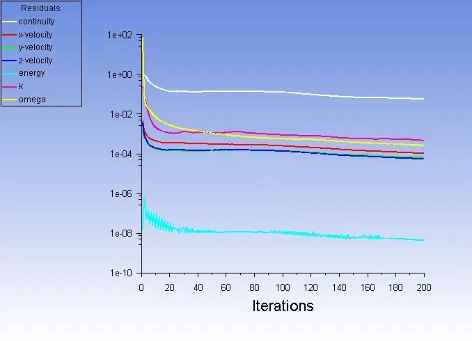
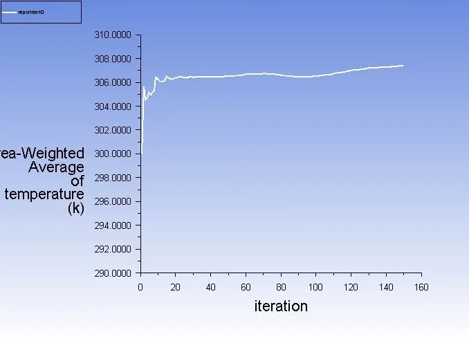
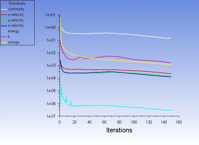
3.To Prove that the simulation has achieved convergence with appropriate images and plots.
4.To Identify potential hotspots on the model.
MODELLING APPROACH:
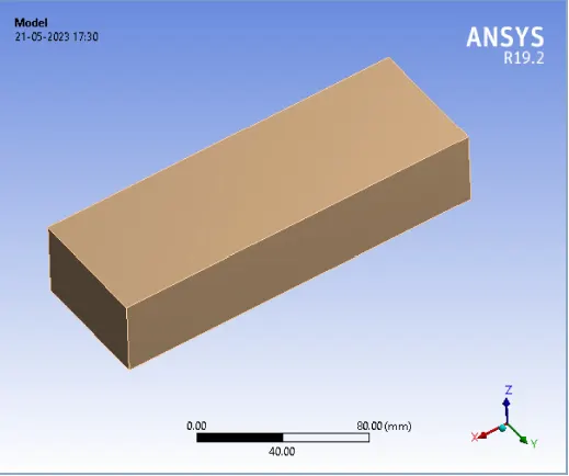
Importing the step file,
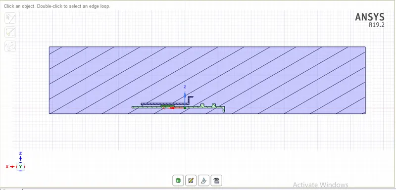
Share the Topology between surfaces,
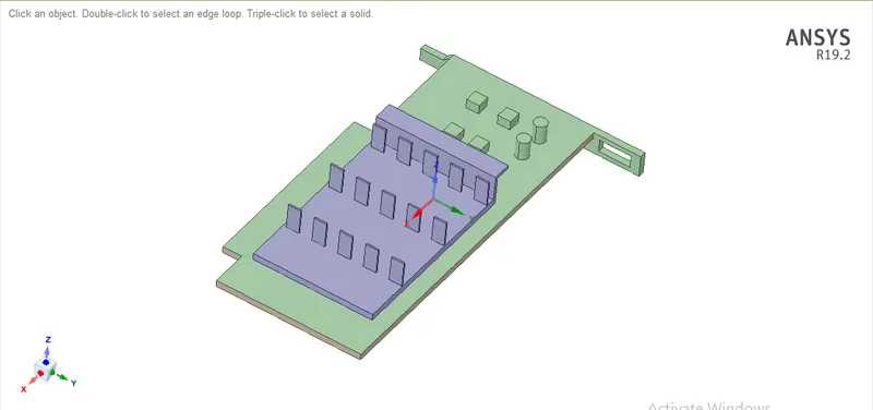
Graphics Card Model,
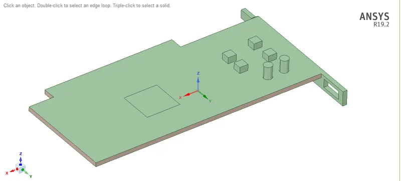
Rename to Base,
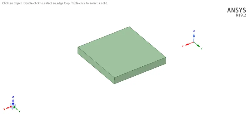
Rename to Processor,
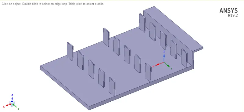
Rename to Fins,
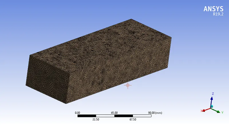
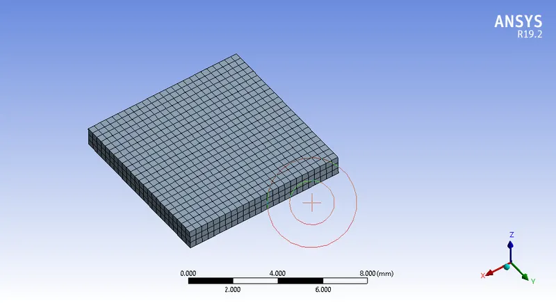
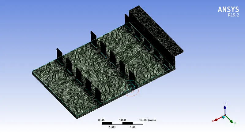
MESHING,
| MESH PARAMETERS | |
| Element size | 2 mm |
| Nodes | 698183 |
| Elements | 4121410 |
Enclosure,
Base,
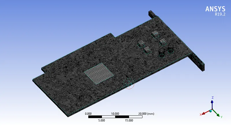
Processor,
Fins,
SOLVER SETUP:
Case 1 - velocity 1m/s, mesh Element size - 2 mm, Energy source Value (considering 1 w) - 1562500 w/m3);
| SOLVER INPUTS | |
| Solver Time | Steady |
| Solver Type | Pressure Based |
| Energy | On |
| Models | |
| Viscous | K - Omega SST |
| Material | |
| Fluid/Enclosure | air |
| Processor | Silicon |
| Fins | Copper |
| Base | Steel |
| Boundary Condition | |
| Inlet velocity | 1m/s |
| Inlet Temperature | 300 K |
| Energy (source terms) considering 1 W output | 15625000w/m3 |
| Iterations | 200 |
| Energy Calculation |
| Length =8mm ,Width = 8mm ,Height = 1mm |
| Energy = p/v |
| P = 1 w |
| V=64mm3 |
| Energy = 15625000w/m3 |
Residual plot,
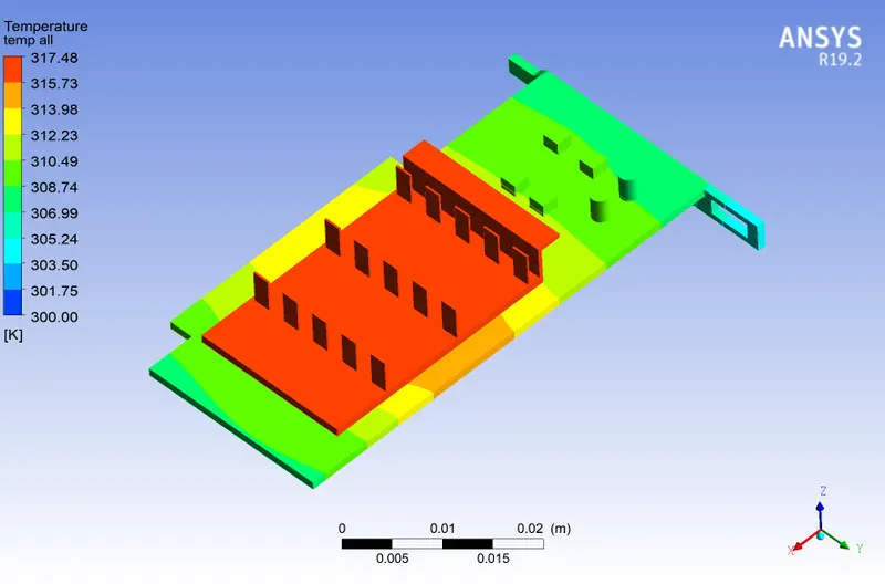
Temperature plot,
Temperature Distribution - All,
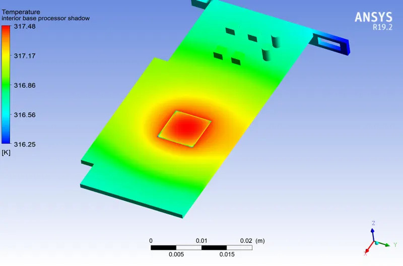
Temperature Distribution - Base,
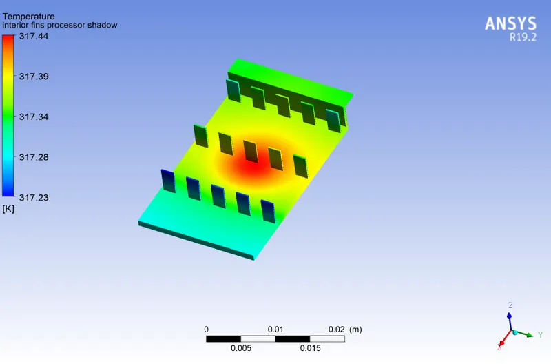
Temperature Distribution - Fins,
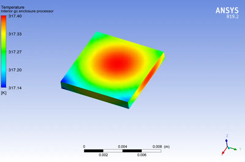
Temperature Distribution - Processor,
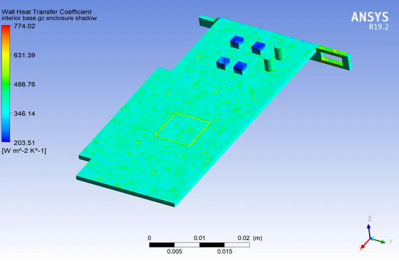
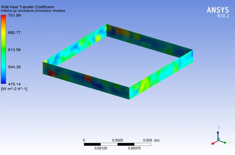
Wall Heat Transfer Coefficient - Base,
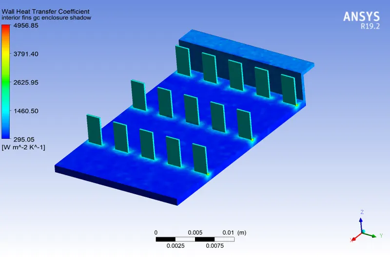
Wall Heat Transfer Coefficient - Fins,
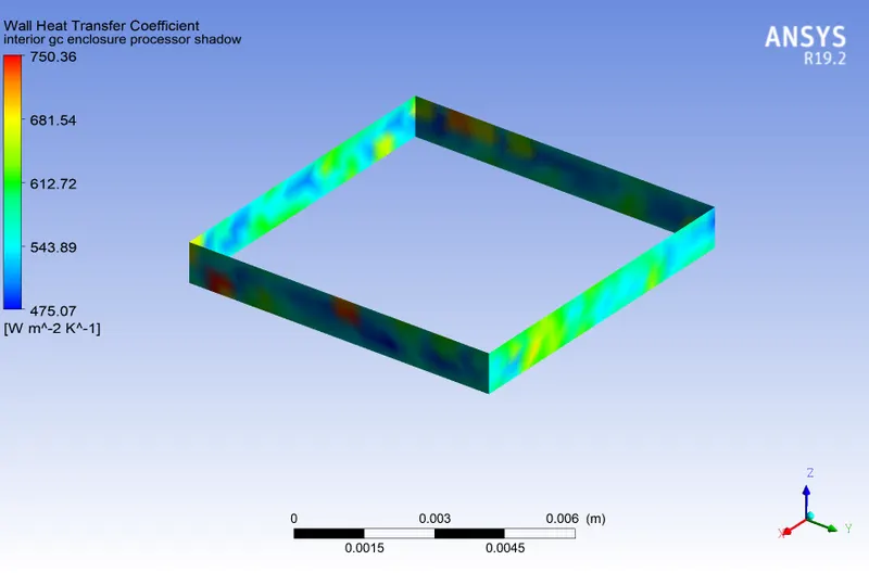
Wall Heat Transfer Coefficient - Processor,
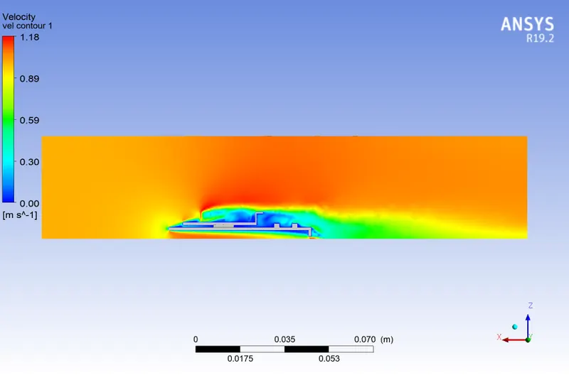
Velocity Contour,
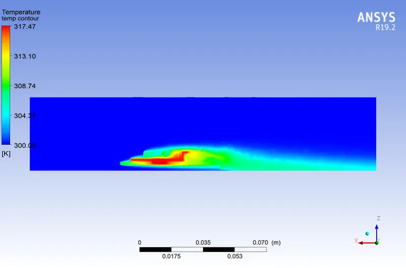
Temperature Contour,
Case 2 - velocity 3m/s, mesh Element size - 2 mm, Energy source Value (considering 65 w) - 1015625000 w/m3)
| SOLVER INPUTS | |
| Solver Time | Steady |
| Solver Type | Pressure Based |
| Energy | On |
| Models | |
| Viscous | K - Omega SST |
| Material | |
| Fluid/Enclosure | air |
| Processor | Silicon |
| Fins and top plate | Copper |
| Base plate | Copper |
| Boundary Condition | |
| Inlet velocity | 3m/s |
| Inlet Temperature | 300 K |
| Energy (source terms) considering 65 W output | 1015625000w/m3 |
| Iterations | 150 |
| Energy Calculation |
| Length =8mm ,Width = 8mm ,Height = 1mm |
| Energy = p/v |
| P = 65 w |
| V=64mm3 |
| Energy = 1015625000w/m3 |
Residual plot,
Temperature plot,
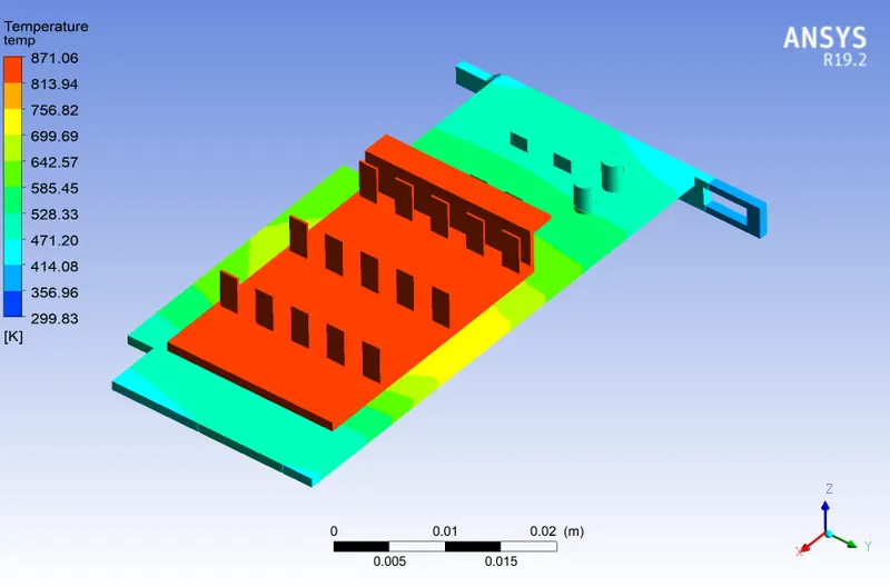
Temperature Distribution - All,
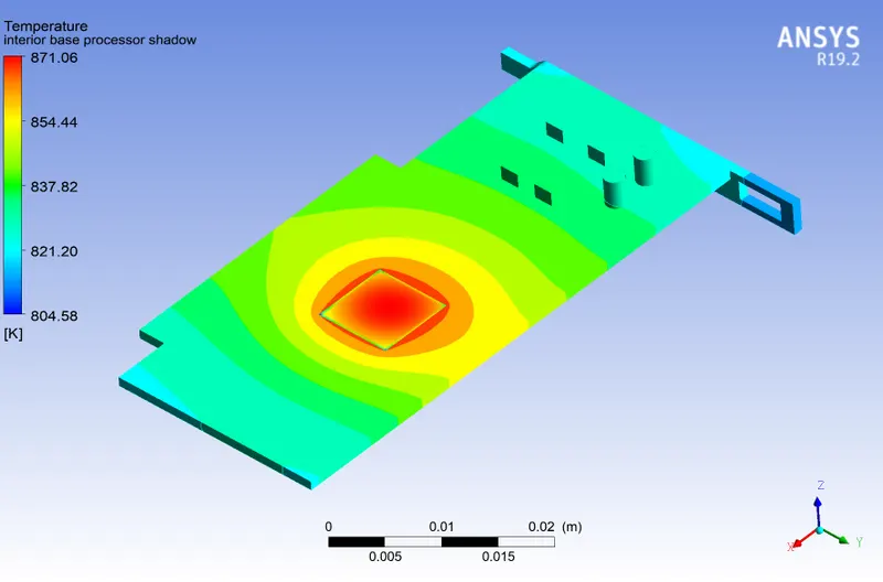
Temperature Distribution - Base,
Temperature Distribution - Fins,
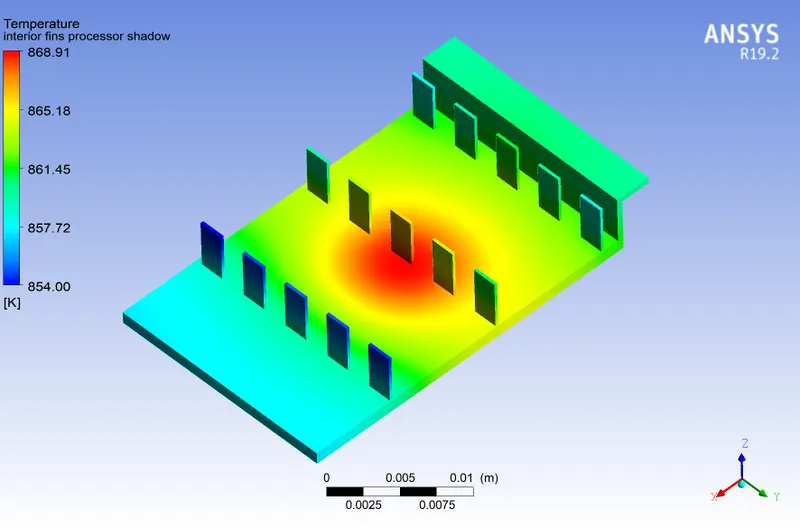
Temperature Distribution - Processor,
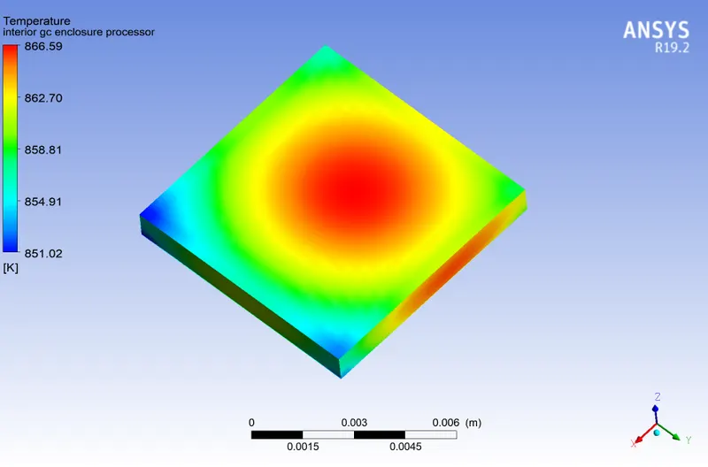
Wall Heat Transfer Coefficient - Base,
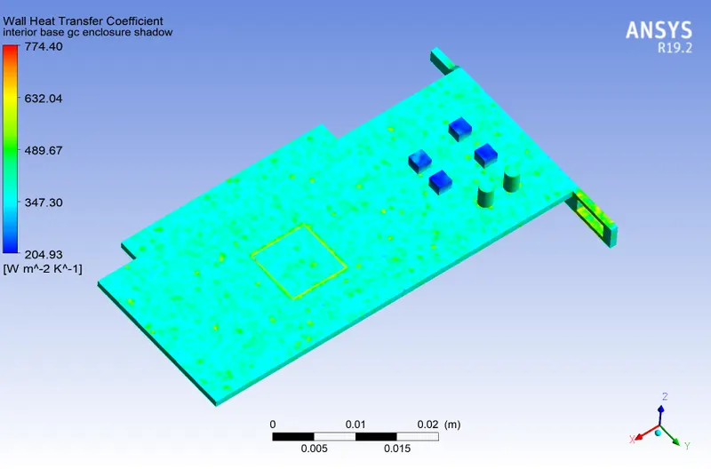
Wall Heat Transfer Coefficient - Fins,
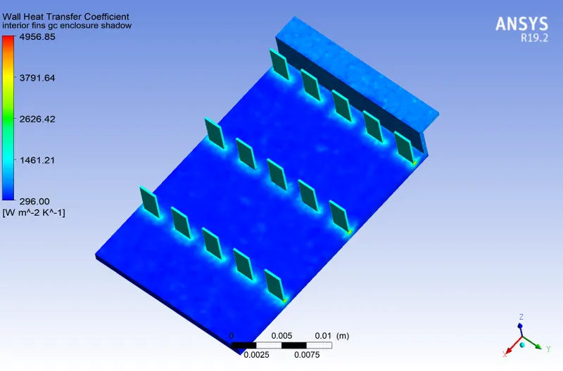
Wall Heat Transfer Coefficient - Processor,
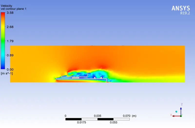
Velocity Contour,
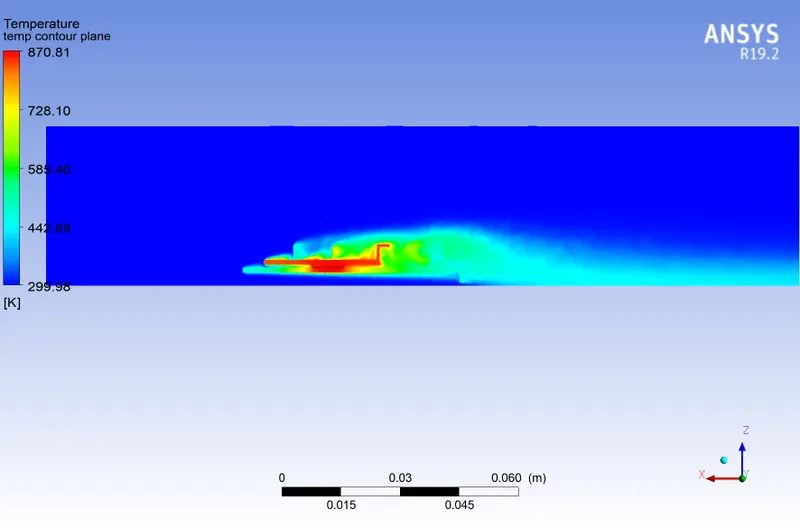
Temperature Contour,
Case 3 - velocity 5m/s, mesh Element size - 2 mm, Energy source Value (considering 65 w) - 1015625000 w/m3)
| SOLVER INPUTS | |
| Solver Time | Steady |
| Solver Type | Pressure Based |
| Energy | On |
| Models | |
| Viscous | K - Omega SST |
| Material | |
| Fluid/Enclosure | air |
| Processor | Silicon |
| Fins and top plate | Copper |
| Base plate | Copper |
| Boundary Condition | |
| Inlet velocity | 5m/s |
| Inlet Temperature | 300 K |
| Energy (source terms) considering 65 W output | 1015625000w/m3 |
| Iterations | 150 |
| Energy Calculation |
| Length =8mm ,Width = 8mm ,Height = 1mm |
| Energy = p/v |
| P = 65 w |
| V=64mm3 |
| Energy = 1015625000w/m3 |
Residual plot,
Temperature Distribution - All,
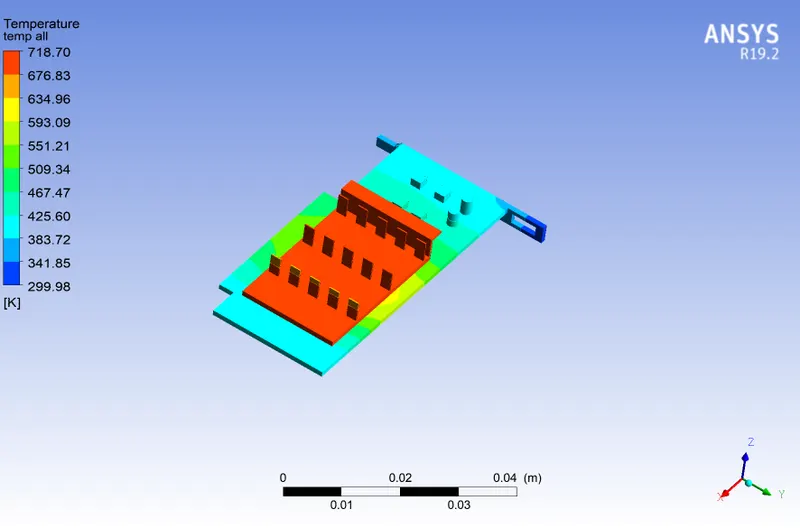
Temperature Distribution - Base,
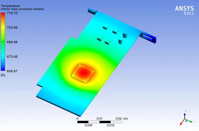
Temperature Distribution - Fins,
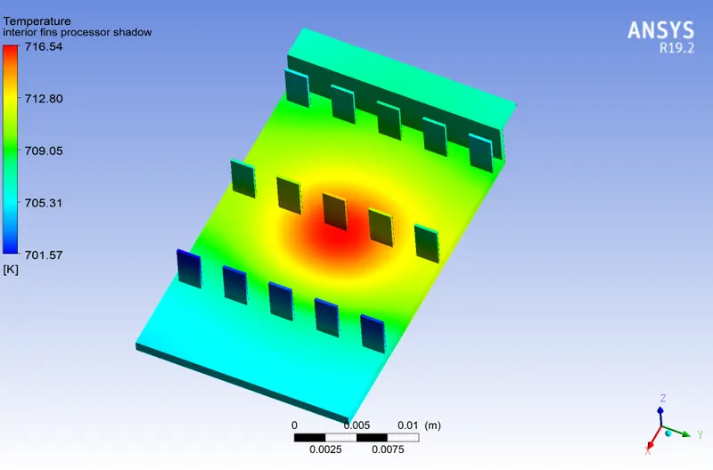
Temperature Distribution - Processor,
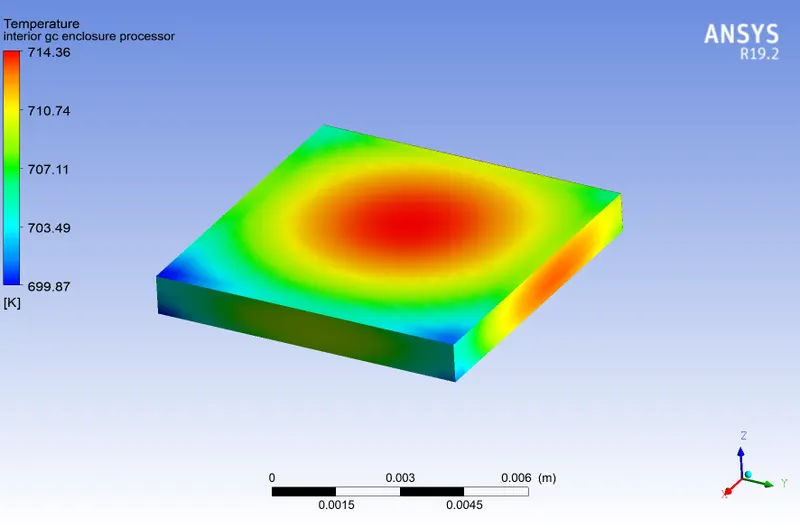
Wall Heat Transfer Coefficient - Base,
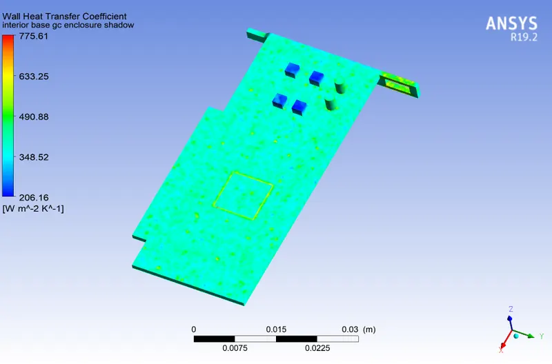
Wall Heat Transfer Coefficient - Fins,
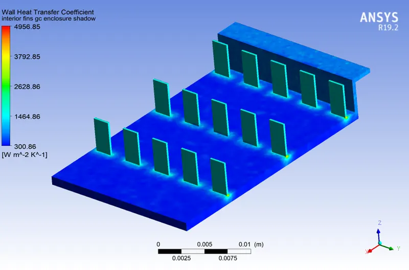
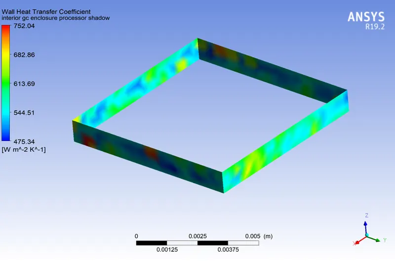
Wall Heat Transfer Coefficient - Processor,
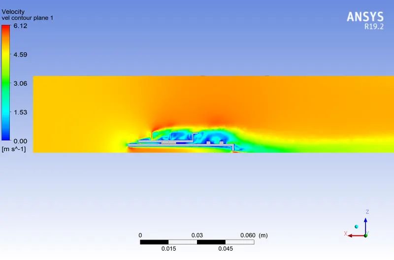
Velocity Contour,
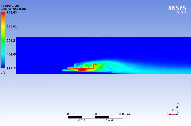
Temperature Contour,
SOLUTION,
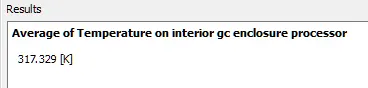
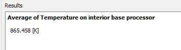
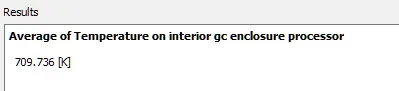
Average Temperature at Processor,
For case 1,
For case 2,
For case 3,
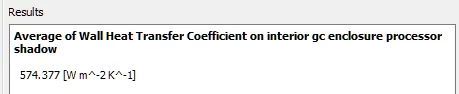
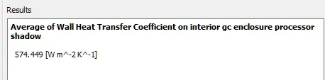
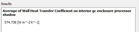
Average Wall Heat Transfer Coefficient - Processor,
For case 1,
For case 2,
For case 3,
CONCLUSION;
Simulation of Conjugate heat transfer on a Graphics card is performed and the temperature distribution at the processor and the temperature plots for different cases created to visualize the results.
In conclusion, the temperature distribution at the processor is low for third case compared to the second case, which clearly shows that the temperature distribution is indirectly proportional to the inlet velocity.
In third case the temperature at the processor is low because of the high inlet velocity which enables the processor to dissipate the heat more quickly than the other cases, this provides quicker cooling of the processor than the other two cases.