Week 6 - CHT Analysis on a Graphics card

Aim:

To perform simulation on graphics card.

Objectives:

1. Run the simulation by varying the velocity from 1m/sec to 5m/sec for at least 3 velocities and discuss the results.
2. Find out the maximum temperature and heat transfer coefficient attained by the processor.
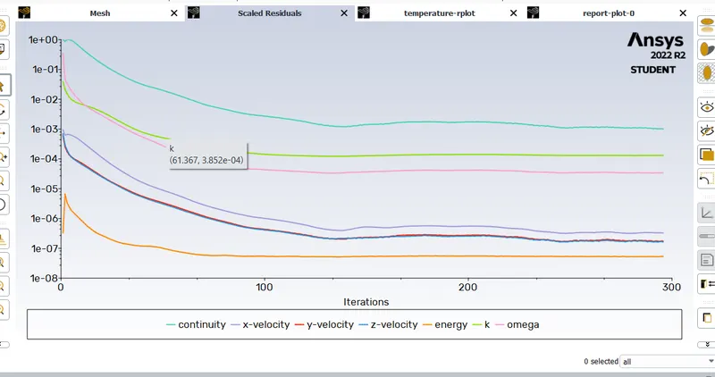
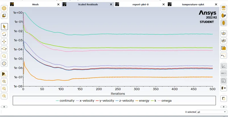
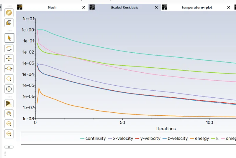
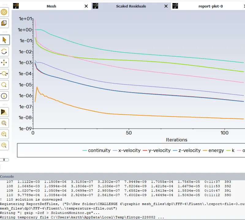
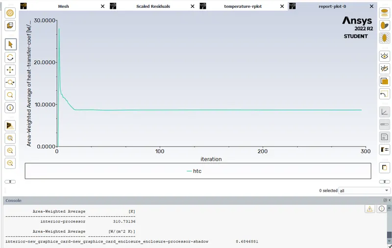
3. Prove that the simulation has achieved convergence with appropriate images and plots.
4. Identify potential hotspots on the model.

Conjugate Heat Transfer anlysis:

 Conjugate heat transfer analysis is based on the mathematical structure problem which describes the heat transfer between the body and the fluid flowing over or inside it as a result of interaction between two objects. At the matching interface, the details are provided for temperature distribution and heat flux along the interface eliminating the need of calculating the heat transfer coefficient.

CHT analysis type allows for the simulation of the heat transfer between the solid and liquid domains by exchanging thermal energy at the interface between them. The simulation of the heat exchangers, cooling of the electronic equipment, and general-purpose cooling and heating system.  In the case of CHT that is being done in this project, we have the convection mode of heat transfer between the fluid and the solid aluminum wall of the exhaust pipe and then the conduction mode of heat transfer is followed within the wall of the exhaust pipe wall.

Model Approach:

1. import geomentry in space claim

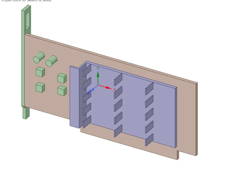
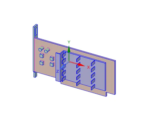
2. prepare the geomentry using share prep option

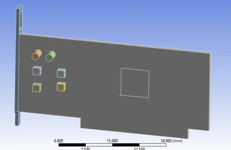
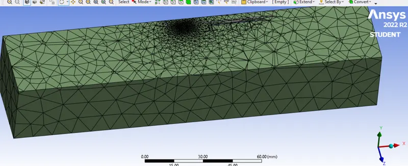
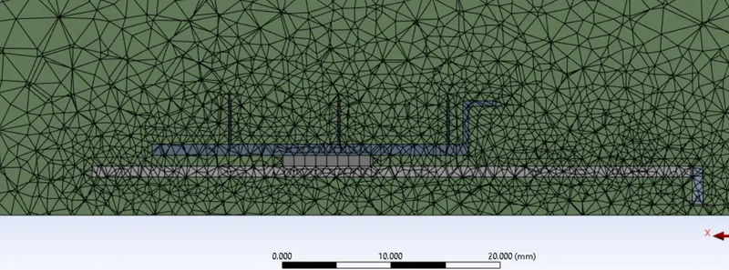
3. open mesh and generate basic mesh size as default size of 10.289mm  and create named selection such as inlet ; outlet ; wall and also name each body as follows

base:

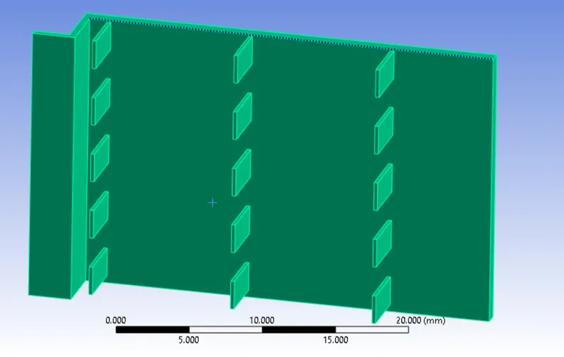
fins:

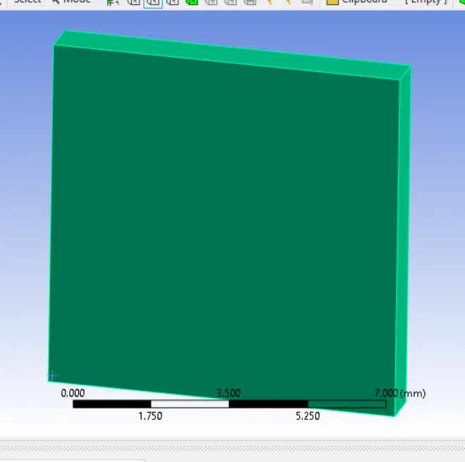
c.Processor:

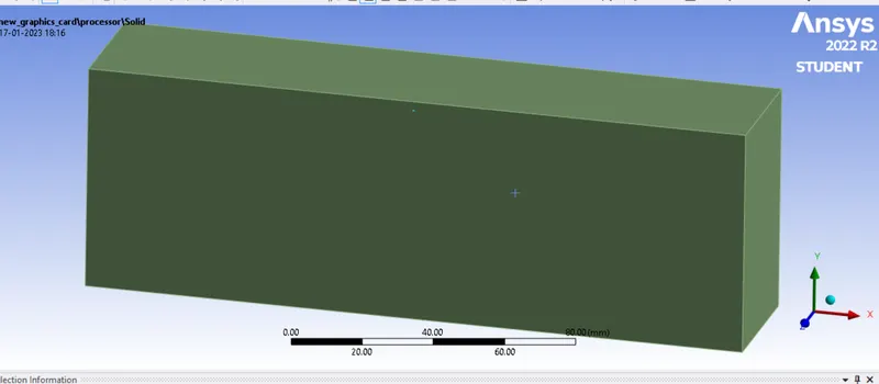
d. Enclosure:

4. open Ansys fluent setup

5. steady state >> viscous>> k-omega>> SST 

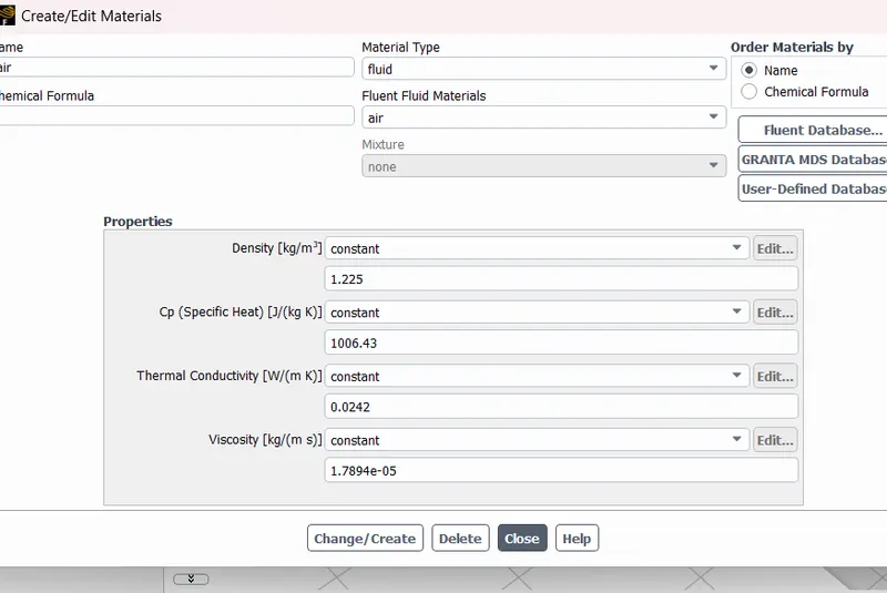
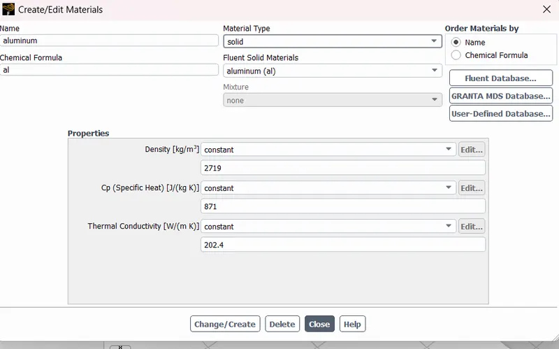
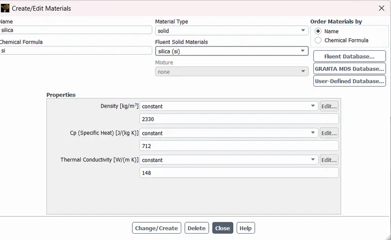
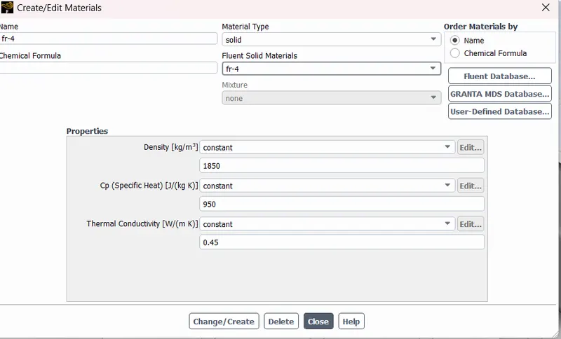
6. create materials as follows

a. Air:

b. Alumunium:

c. Silicon:

d. FR4

7. turn on energy equation:

8. set boundary condition as inlet with 5m/s velocity and 300k temp ; make outlet as 0Pa gauge pressure 

9. set cell zones material as follows

a. base >> FR4

b.fins >> Alumunium

c. enclosure >> air

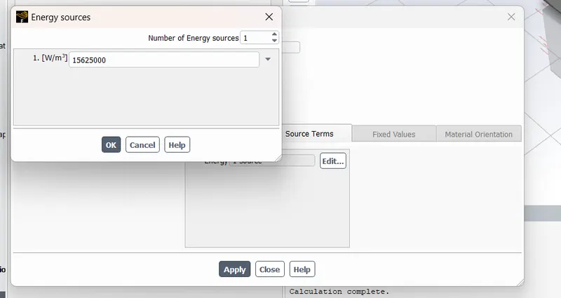
d. processor >> silica >> turn on energy souce as 15625000 W/m3

note:

here we have taken graphic card processor as 1W

volume of processor = 8*8*1= 64mm3 = 64 x 10^9 m3

hence Heat generated= 1/(64 x 10^9)= 15625000 W/m3

8. also iniltialize the simulation and turn on plots for temp on processor and  Heat transfer coefficient of  processor and run it for 500 iterations.

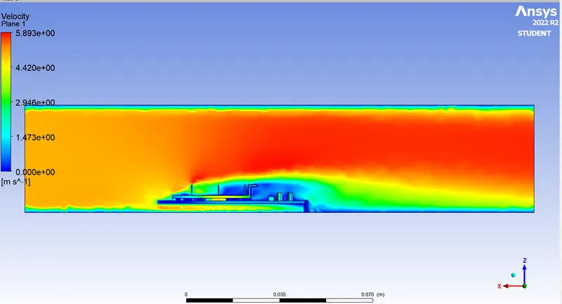
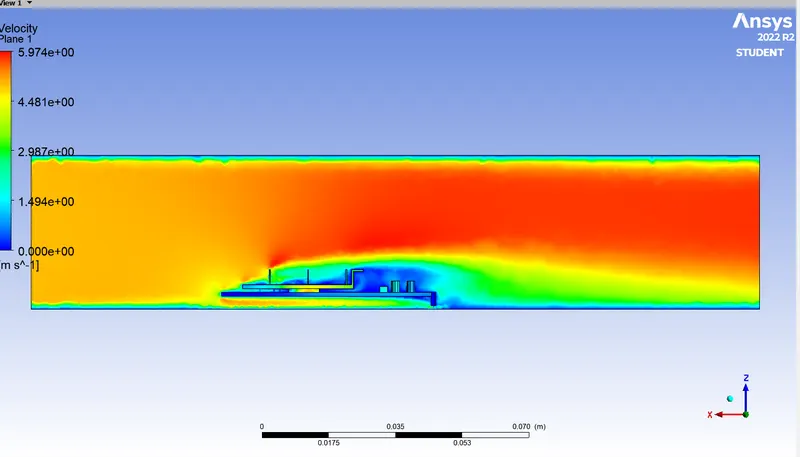
9. go to cfd post  and turn on heat distribution over components of graphics card and Also take mid plane and plot contours for velocity and temperature along the air flow.

10.  analyze the base mesh which seems not  fine on contour

11. then repeat simulation for two differnt finer mesh 

12. then repeat simulation for  another two different velocities for last finer mesh and anayze it

observation:

contents	base mesh	case 1	case 2	case3	case 4
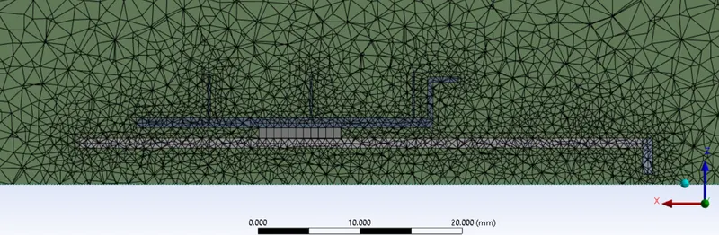
element size	default value (10.289mm)	overall size 3mm other components 1mm	overall size 2.5mm other components 0.75mm	overall size 2.5mm other components 0.75mm	overall size 2.5mm other components 0.75mm
no of elements	81427	226580	404687	404687	404687
mesh
velocity	5m/s	5m/s	5m/s	3m/s	1m/s
residuals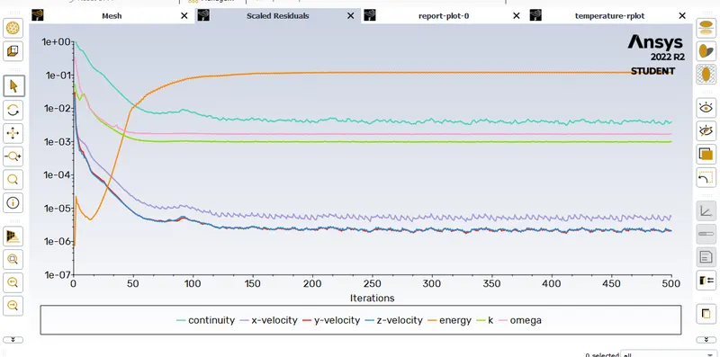
temp plot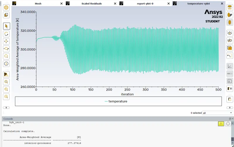
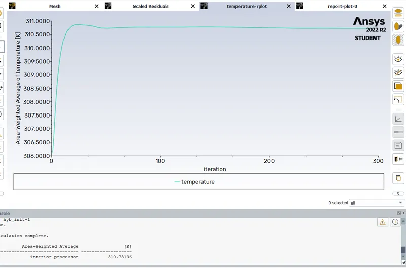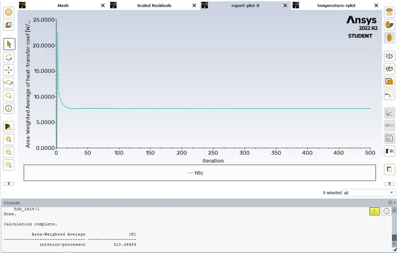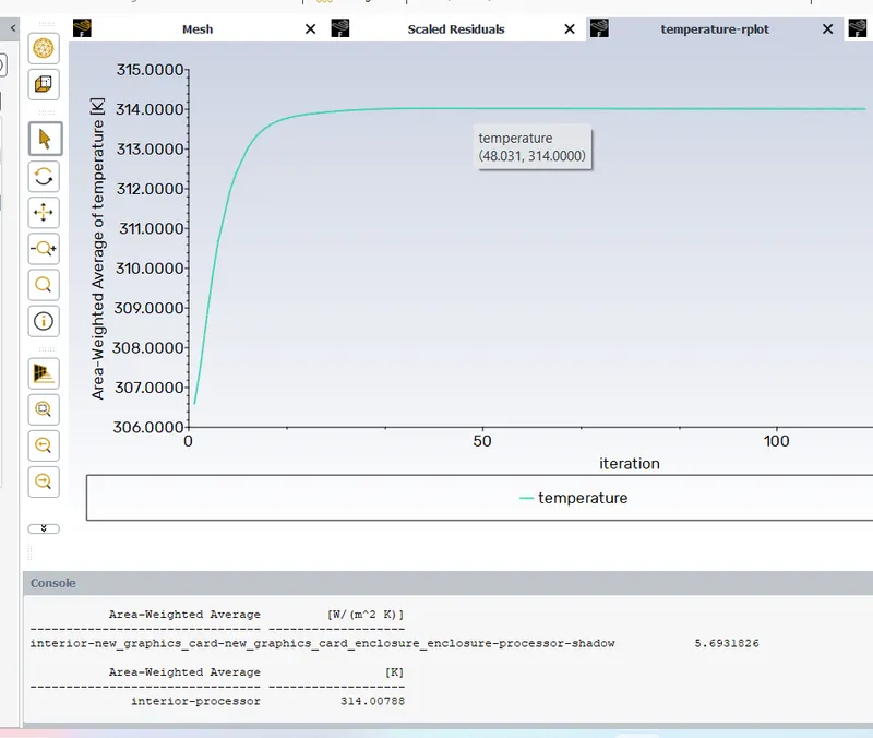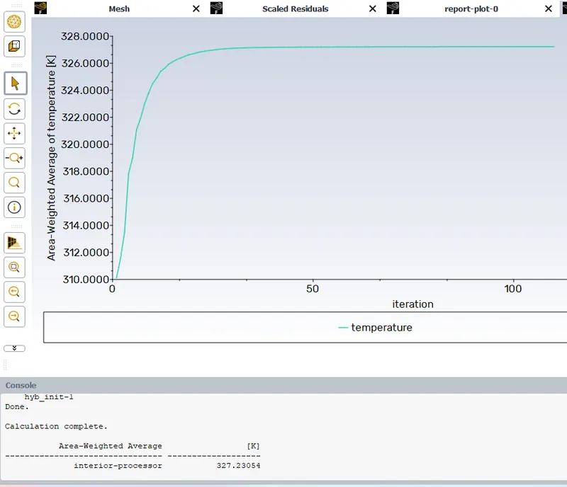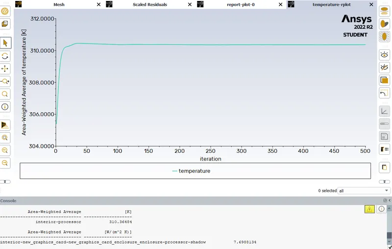
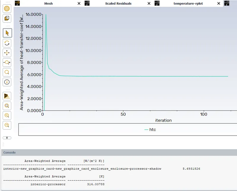
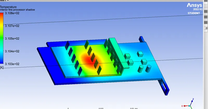
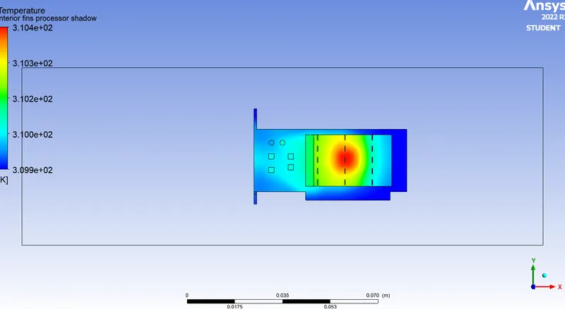
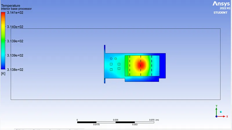
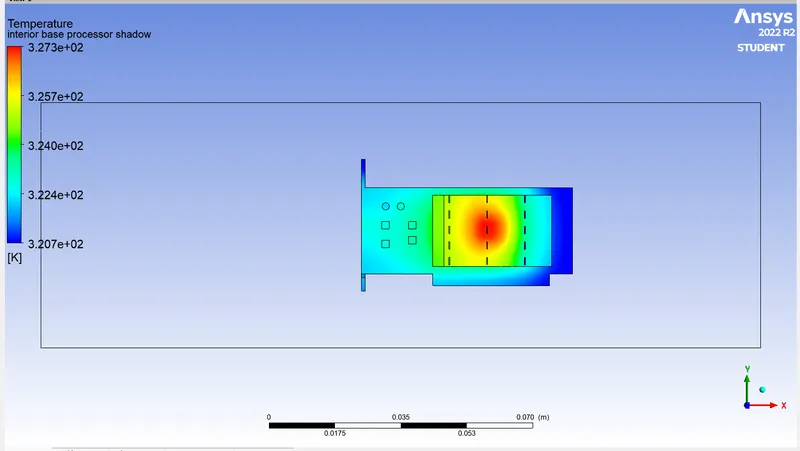
temp attained	277.37K	310.73K	310.36	314.007	327.23K
htc plot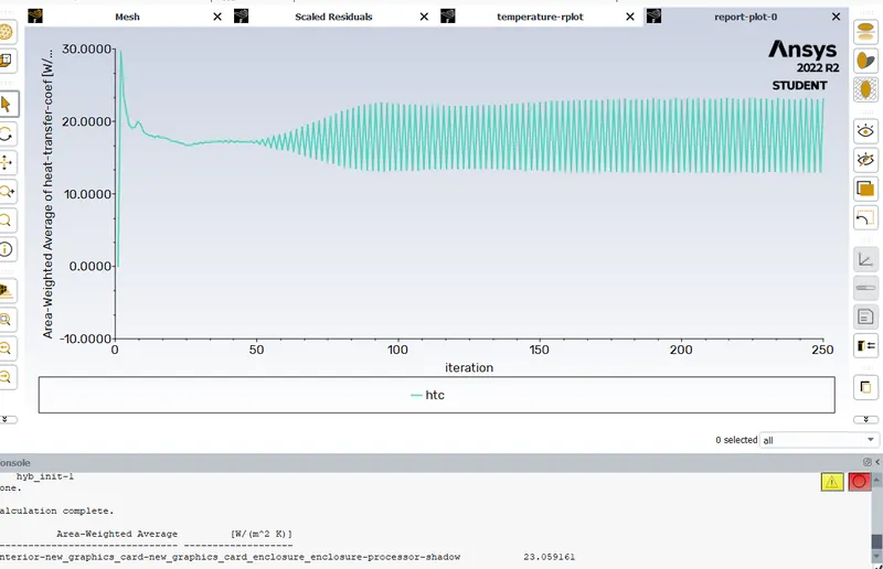
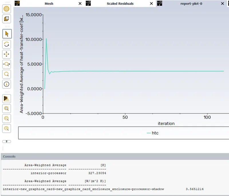htc attained	23.05 W/m2K	8.68 W/m2K	7.699	5.69 w/m2K	3.56 W/m2K
velocity along plane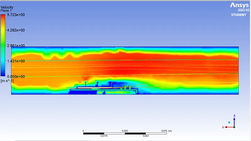
temp along plane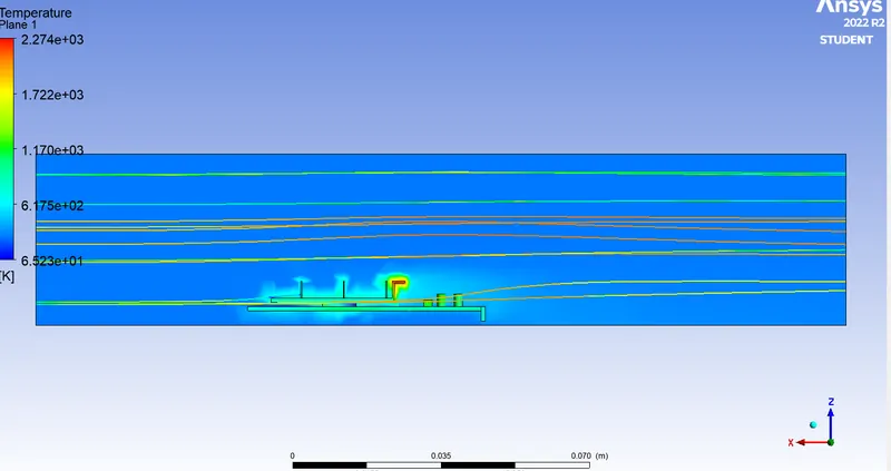
vector plot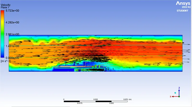
overall temp distribution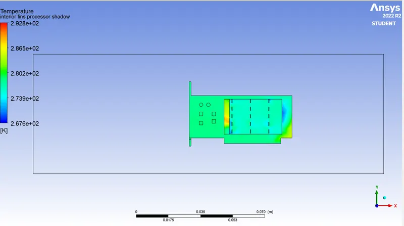
temp around processor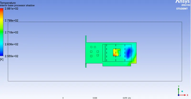

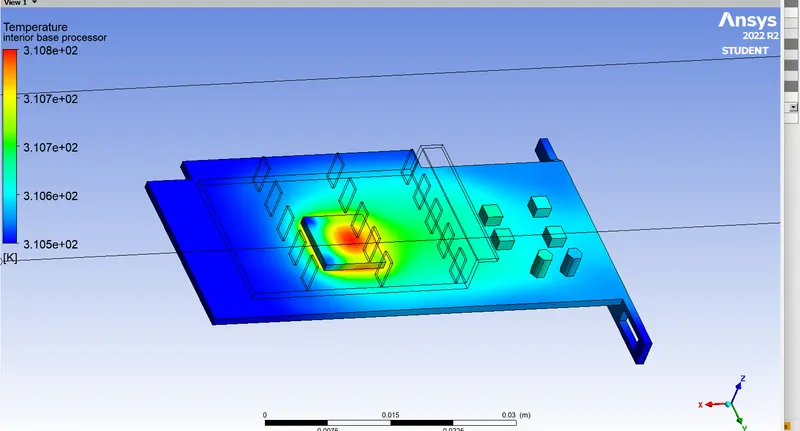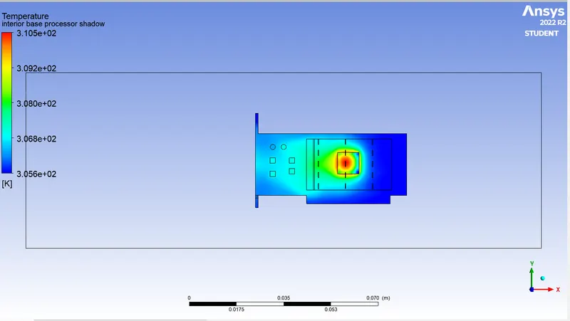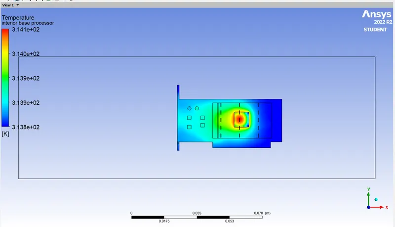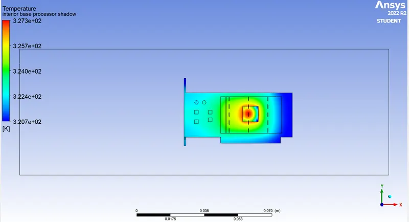points observed:

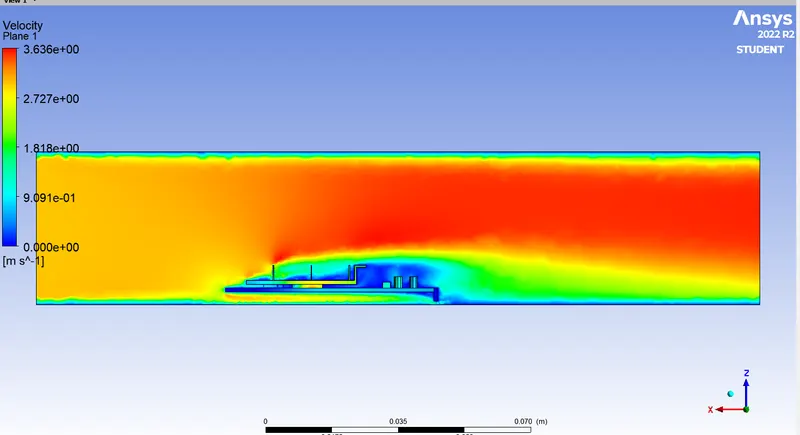
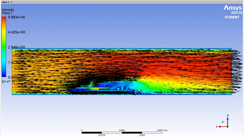
•  first lets see base mesh which was not so perfect and also it doesnot show results based on real world applications the reason behind this is we took mesh size as common which doesnot suits for components with less than 5mm so in other cases i need to provide different mesh size for components and enclosure
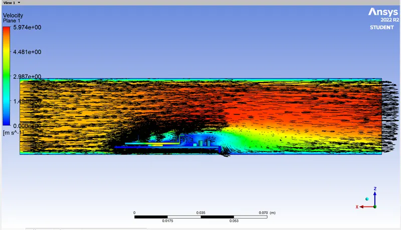
• next cases i observe it to be more exact results such that heat is generated on processor ( we can observe it from contours as well)
• on the next case we can observe that it is more clear and also results are good 
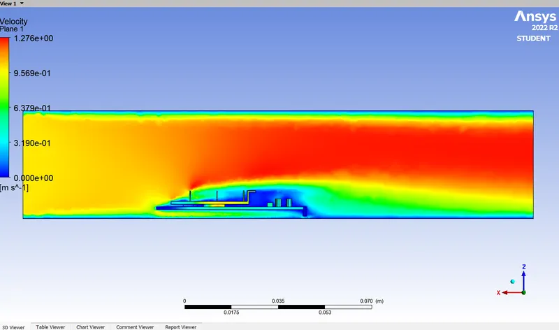
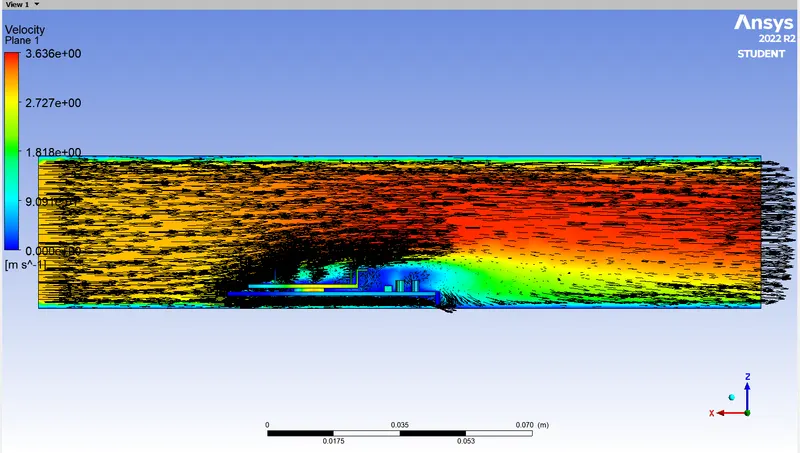
• on the next cases we perform on the same mesh but with differnt velocities such that we reduce it for 3 and 1 m/s
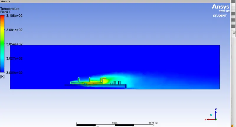
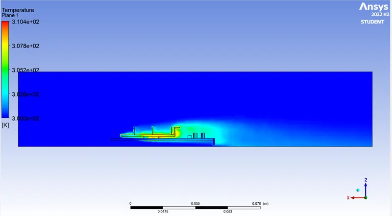
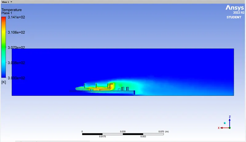
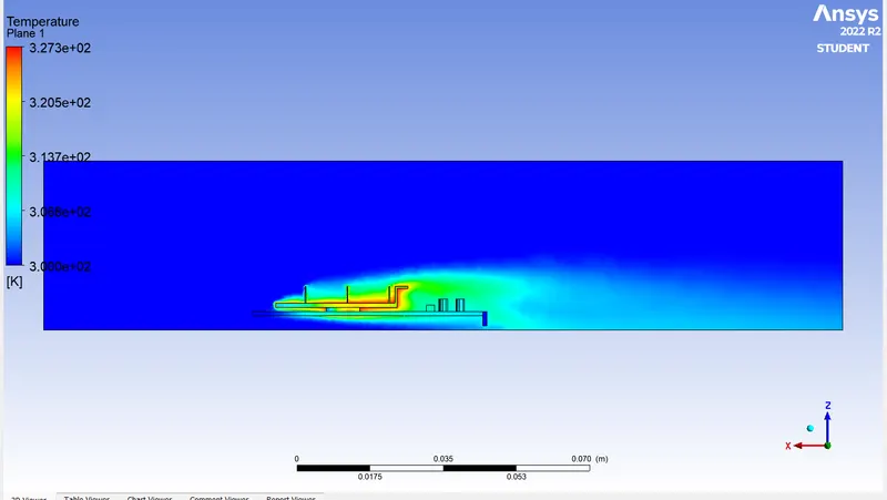
• while observing it is clear that due to reduced velocities temp distribution areas are minimum for simulation with lower velocities also more heat is generated too.
• while comparing the max temp developed on processor for each cases it is sure that lower velocity cases produces more heat 

Results:

Thus we performed simulation on htc for two different mesh size with three differnt velocity and observed as follows

1. lower the velocity the temp will be high because the heat is not carried away by the air due to low velocities.
2. lower the mesh size exact simulation can be gained properly.