Week 6 - CHT Analysis on a Graphics card

AIM

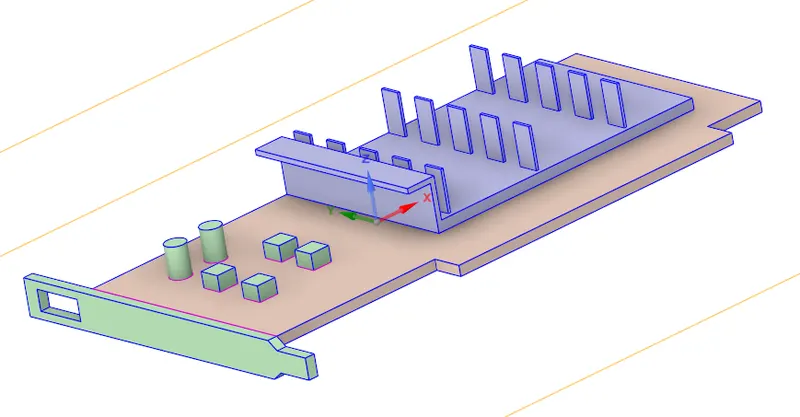
To perform a steady-state conjugate heat transfer analysis on a model of a graphics card, properly define the correct solid and fluid zones, run the simulation with combination of coarse and refined mesh for different regions and also by varying the velocity from 1m/sec to 5m/sec for 3 different cases, find out the maximum temperature and heat transfer coefficient attained by the processor and identify potential hotspots on the model.

INTRODUCTION

Conjugate heat transfer (CHT) analysis is an analysis performed to analyze the heat transfer between solids and fluids. As we know that the mode of heat transfer in solids is conduction and in fluids it is either due to free or forced convection, it becomes necessary to study the behaviour of the fluids so as to understand various parameters like temperature, pressure, velocity, etc.

A classic example of CHT is the transfer of heat from the heated spoon to the atmosphere until thermal equilibrium is reached. Here, the heat first conducts through the spoon to the top surface and then through natural convection it is transfered to the atmosphere. Using a proper mesh size, we can simulate the flow of heat and thus study various parameters like temperature, velocity, etc.

In the current project, CHT analysis is performed on a model of graphics card using ANSYS Fluent. Two different mesh sizes and three different velocities are used for the analysis:

1. Baseline mesh of 10 mm and velocity of 1 m/s
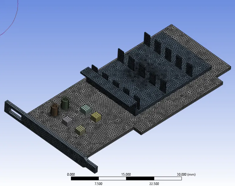
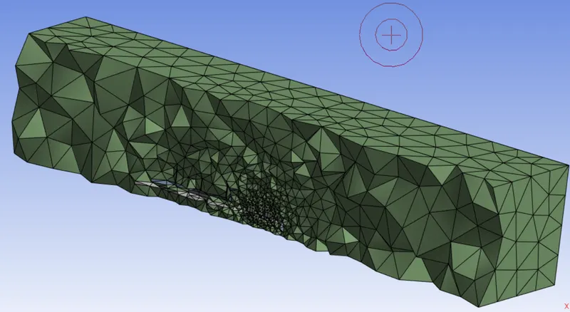
2. Refined mesh of face sizing 500 mm for the outer enclosure, body sizing of 0.3 mm for processor, 0.6 mm for fins and 0.8 mm for PCB and velocity of 3 m/s
3. Refined mesh of face sizing 500 mm for the outer enclosure, body sizing of 0.3 mm for processor, 0.6 mm for fins and 0.8 mm for PCB and velocity of 5 m/s

PREPARING THE GEOMETRY AND PRE-PROCESSING

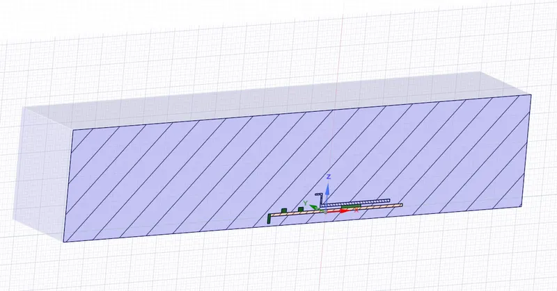
After importing the given model in the Spaceclaim, we first extract the internal volume and then share the geometry so that there will be a relation maintained between the the various geometries and this would help in meshing.

Since we know that the processor generates large amount of heat, we use fine mesh near the processor, fins and board to capture the properties for the solid and fluid components. For the outer enclosure we use coarse mesh.

SOLVING APPROACH

For both baseline mesh and refined mesh, the three dimensional Navier-Stokes equations are solved using a steady state pressure-based solver. For modeling turbulence flow the K-omega SST model is employed since we are not interested in capturing the parameters at the walls and also there is no no-slip flow.

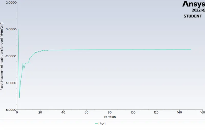
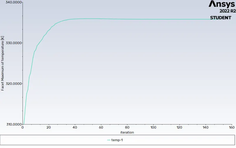
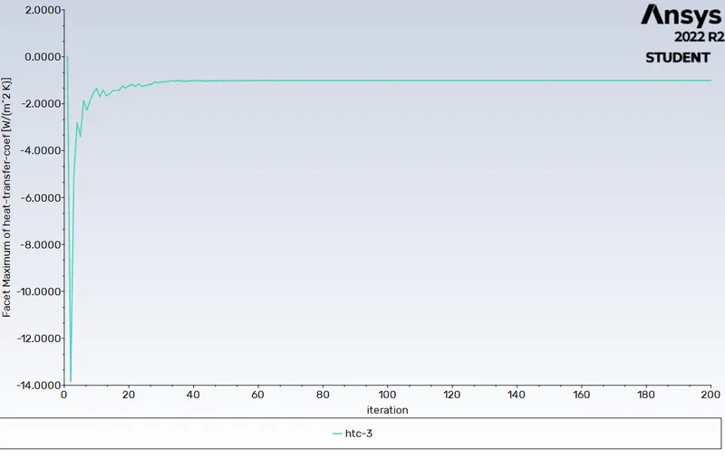
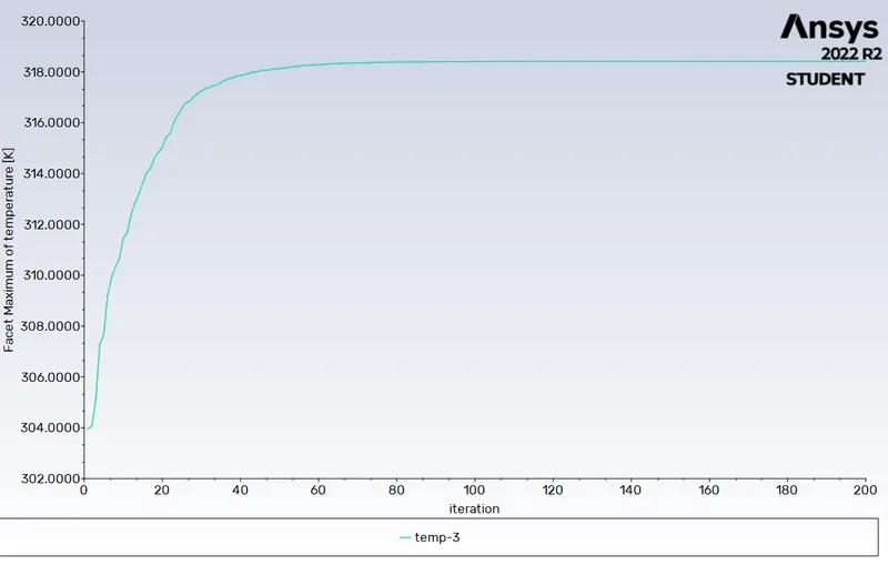
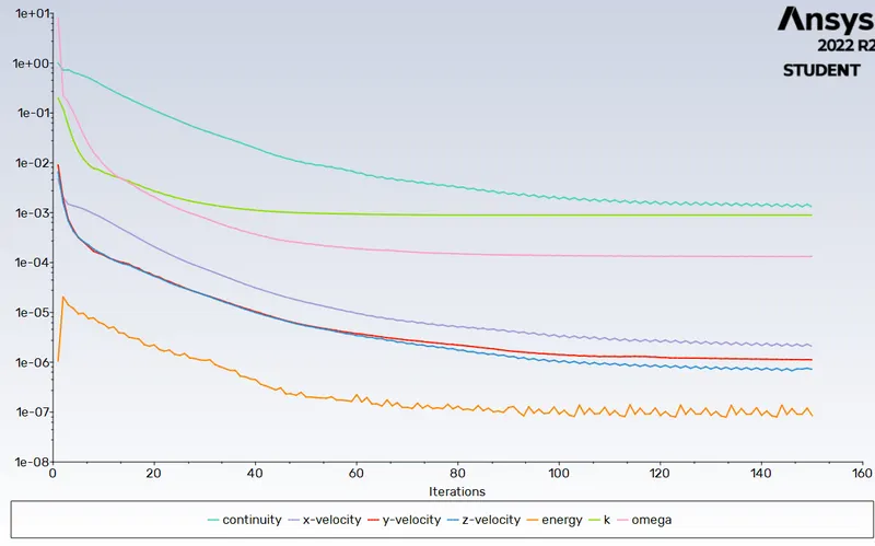
The solution is initialized using a hybrid initialization scheme and different velocity boundary conditions are applied for all the cases. For both the cases the solver is run for 150 iterations since it is sufficient enough to get the converged solution. Maximum temperature and HTC are computed from the plots. Temperature and velocity contours are plotted for all the cases.

RESULTS

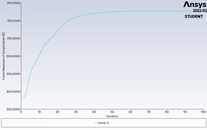
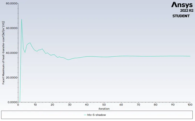
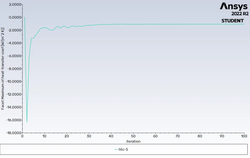
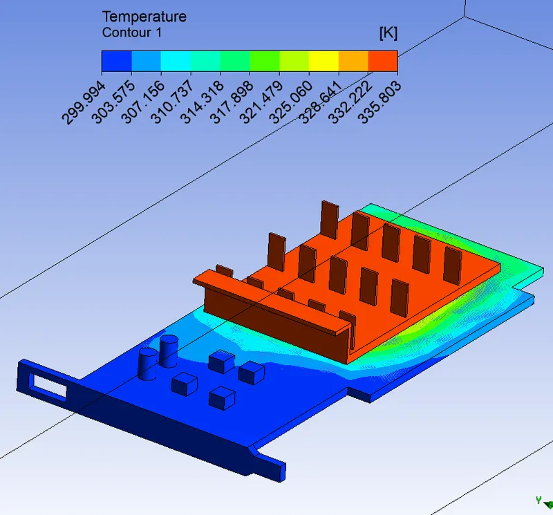
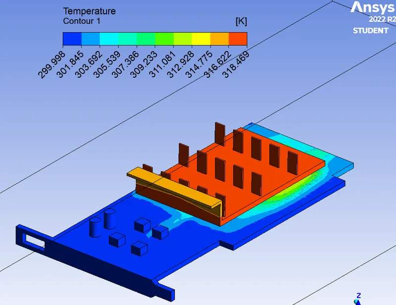
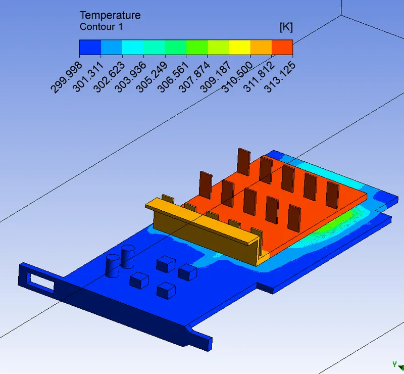
1. Simulation results (HTC and temperature plots) for three different velocities of 1,3,5 m/s

Case 1

Case 2

Case 3

2. Residue plot to prove that the simulation has achieved convergence

3. Maximum temperature and heat transfer coefficient attained by the processor

Velocity (m/s)	Max HTC for processor (W/m2K)	Max HTC for processor shadow (W/m2K)	Max Temp (K)
1	-1.52	3.35	335.8
3	-1.09	25.9	318
5	-1.077	37.22	313

4. Potential hotspot on the given model - Processor

Ideal GPU hotspot temperature is 80C-95C, and it shouldn’t be below 45C, but maximum temperature differs from one GPU manufacturer to another because of the difference in the placement of the thermal sensors.

CONCLUSION

From the above table of results we can conclude that by increasing the velocity from 1 m/s to 5 m/s the heat transfer coefficient increases and temperature reduces, but there is not much variation in the temperature for velocity of 4 m/s and 5 m/s and thus by increasing the velocity using external sources, increases the cost of the set-up. Thus the optimum velocity is between 3 and 4 m/s to achieve the desired reduction in the temperature.