Week 6 - CHT Analysis on a Graphics card

Aim:

To perform a steady-state conjugate heat transfer analysis on a given model(graphics card).

Objectives:

• To run simulation and discuss results by varying velocity from 1m/s to 5m/s for atleast 3 velocities.
• To find Maximum temperature(facet maximum) and Heat transfer coefficient attained by the processor.
• To prove simulation has converged and to attach required plots with it.
• To identify potential hotspots on the model.

Conjugate Heat  Transfer provides the temperature prediction and the hotspot regions at the solid-fluid interface and we can also predict the heat transfer accurately. Eg. Conduction through solids, convection through fluid, and thermal radiation

Introduction

CHT (Conjugate Heat Transfer) analysis is based on a mathematically structured problem, which describes the heat transfer between a body and a fluid flowing over or inside it as a result of interaction between two objects.

Conjugate heat transfer (CHT) simulations, which involve both fluid and solid domains within a CFD calculation, come with their own set of complications. This includes the solver's capability for handling and connecting thermal information between fluids and solids, as well as the workflow’s capacity to handle different thermal inertias.

The details are provided for temperature distribution and heat flux along the interface eliminating the need of calculating the heat transfer coefficient. Moreover, the heat transfer coefficient can be calculated later.

One of the simplest ways to realize conjugation is through numerical methods.

Application:

The CHT methods have become more powerful tool for modelling and investigating natural phenomena and engineering systems in different areas.

CHT in recent years has significantly improved the cooling performance of electronic equipment such as the design of heat sinks and the design of heat exchangers for the waste treatment plant. One such application of CHT is Graphics card in electronic systems.

In this challenge, we are going to perform steady-state conjugate heat transfer analysis on the given graphics card model, and to understand conduction & convection of a processor is considered and heat transfer coefficient and maximum temperature is measured for the processor. In this challenge we consider processor as a source term with 1kW as power. The model given is meshed as coarse and finer mesh to find the differences of the results we get with those meshes and can conclude which mesh will be better to perform and get better results.

Solving and Modelling approach:

• Spaceclaim is opened and the given model is imported with it.

Graphics card:

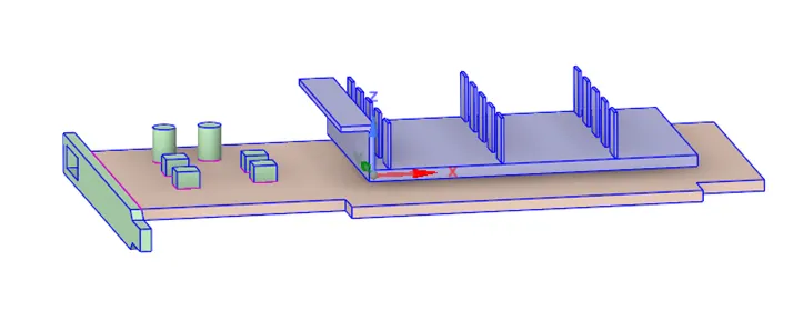
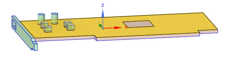
Base of the model – Graphics card:

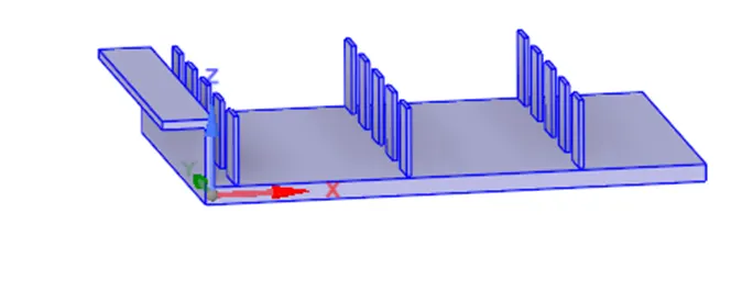
Fins of Graphics card model:

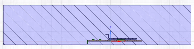
• Entire Graphics card is enclosed in a domain we named it as enclosure

Before moving into meshing process, we need to share topology in spaceclaim so that we can obtain a better mesh.

Pre-processing:

In our challenge we have to perform coarse mesh and finer mesh for a conclusion that which mesh gives us a better result.

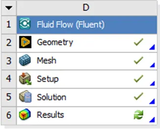
* For coarse mesh - we open mesh by right clicking on mesh and select edit on it to open mesh window 

 

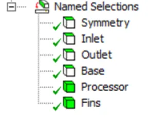
* After opening mesh we name parts for reference by selecting a face/body and right click and select create named selections or press N as shortcut key to name selected faces.

* Then click on Mesh and click on Generate mesh. A coarse mesh will be generated. Then close Mesh and update the mesh.

For Refined Mesh, we have applied Body sizing to the Processor hence we need more details on and near Processor.

Body Sizing on Processor = 0.5mm

Mesh size is set to 2mm.

Mesh is done as coarse and finer for the simulation as two cases.

After completion of the mesh process, we are ready for the numerical simulation and be performed using Ansys Fluent which is a CFD simulation software.

In this challenge we are performing internal flow and it is steady state simulation.

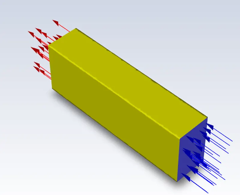
When opening Fluent, Mesh is imported to it, to check if any distortion happened while importing , before starting the setup check the mesh.

Setup(Solver setting):

*Solver type is Pressure based as we are performing simulations with smaller velocities 1,3,5m/s.

*Energy is turned on, as we are working on the challenges regarding heat transfer energy.

*Viscous model is set as a K-omega and SST turbulence model.

*Materials are created in solid category to assign to the Fins, Processors, Base and for the domain – fluid as air is assigned.

*Boundary condition – inlet as velocity, there are 3 different velocities 1,3,5m/s and Temperature is set to 300K, inlet and outlet as pressure-outlet , Domain as Symmetry so that we can reduce computational power needed

*Cell zone conditions

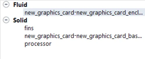
Fins set to aluminium as its material as it conducts heat, Base is set to plastics because usually boards are quality plastics and it insulates heat.

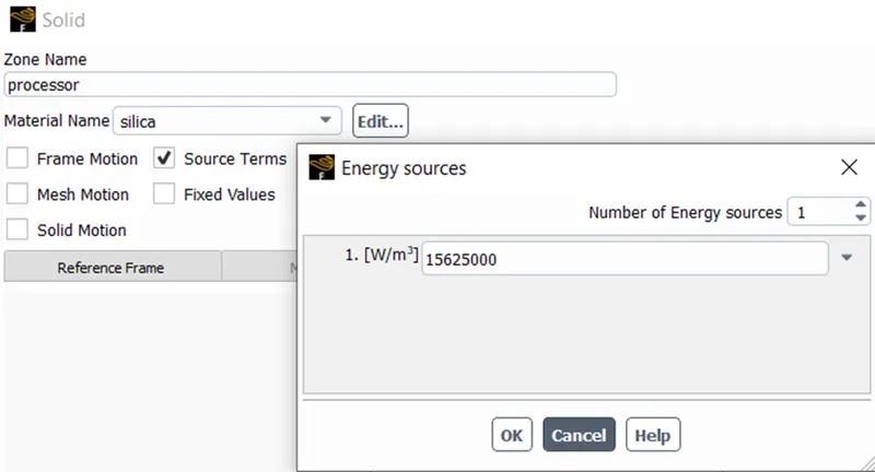
Processor is set to Silica and processor acts as a Source of 1kW in this challenge and when calculated to Energy = power/volume, we get 15625000 , as volume is 8x8x1.

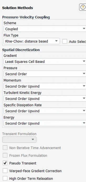
In Methods are set as default settings for K-omega model,

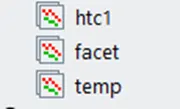
Before initialization, as we need some plots like heat transfer coefficient, facet maximum(maximum temperature), Average temperature

We created Report Definition for those,

Initializing method as Hybrid Initialze, and initialized the problem with imaginary values.

No.of iterations are given and calculation is started.

Result:

Results that need to be attained are Heat transfer coefficient, maximum temperature and plots to show convergence.

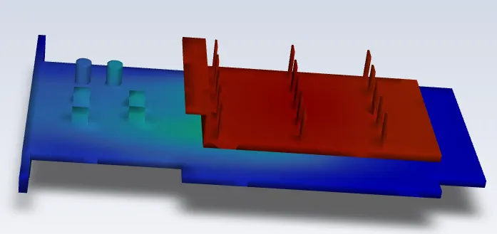
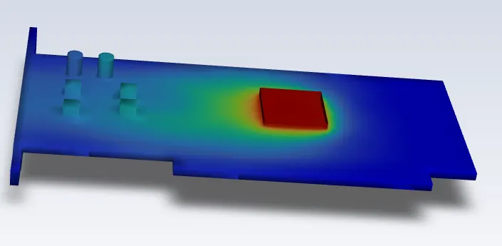
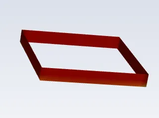
In this model, Processor generates heat and it acts as a Source. Heat generated is both convected and conducted, heat is conducted to the Fins made of aluminium and Convected from the sides of the Processor, because top of the processor is attached to the Fins and Bottom to the Base.

The above figure shows the conduction of heat to the Fins, Sides where heat convects is shown below,

Plots:

	For Refined mesh(5m/s)	For Coarse mesh(5m/s)
Heat Transfer       coefficient
Maximum  Temperature
Area weighted Average - Temperature

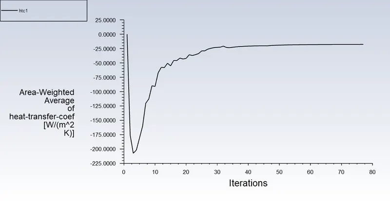
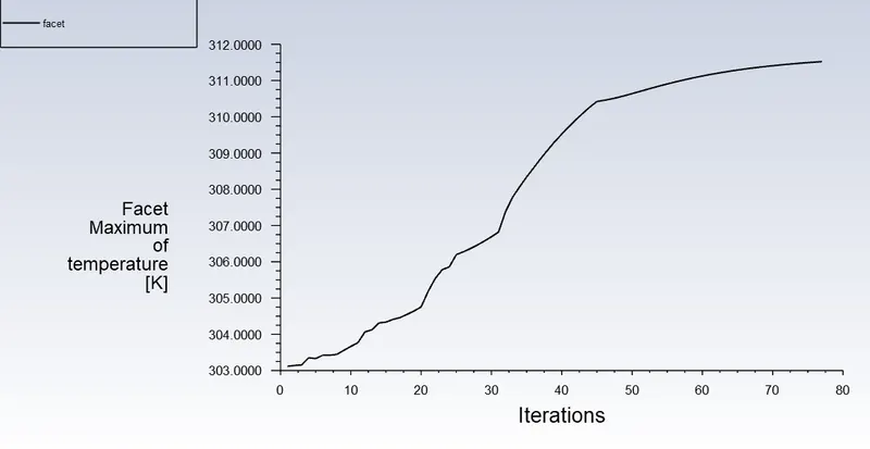
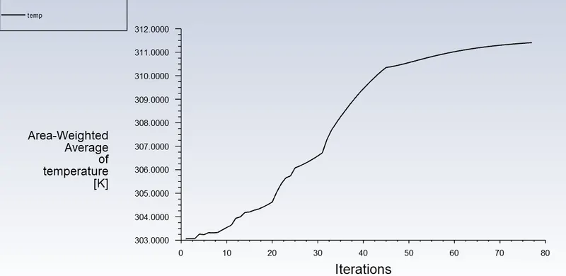
 For Coarse mesh(5m/s),

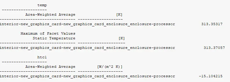
For Refined mesh(5m/s),

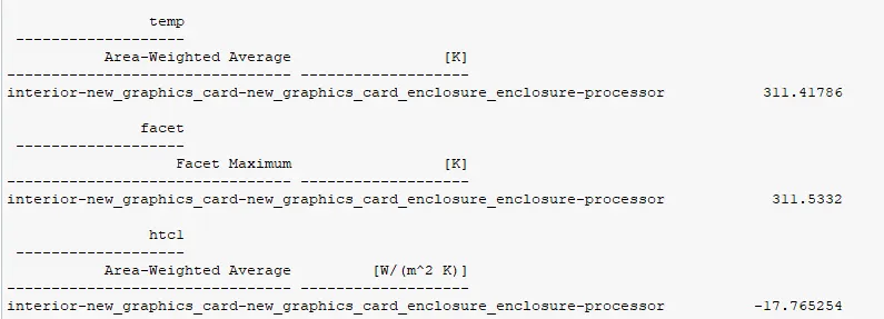
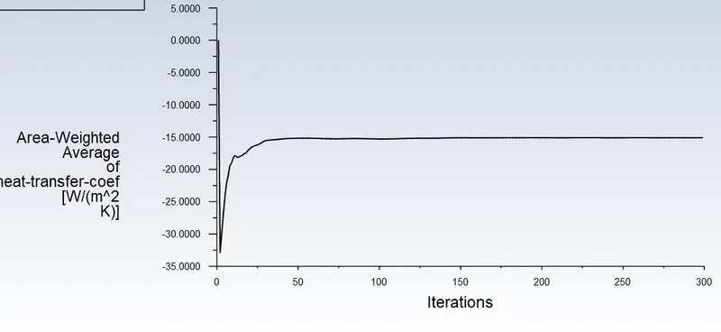
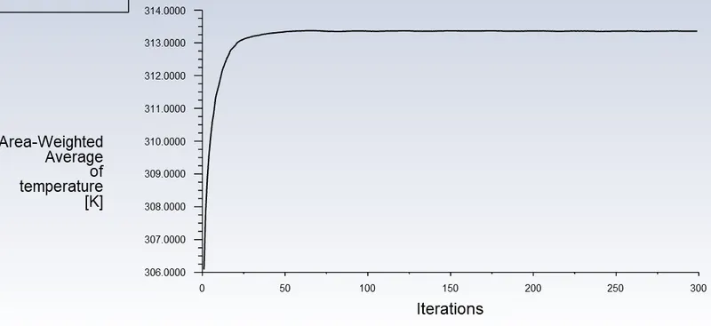
 When compared between Coarse and Refined mesh, there is no much difference in the results, but when when between accuracy and convergence of the simulation, Refined mesh has better accuracy and for further simulation for the velocities 1,3m/s we can opt Refined mesh model to further proceedings

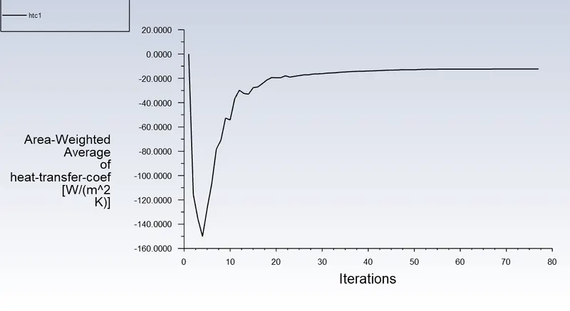
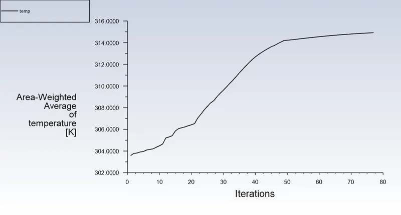
For Refined mesh(3m/s),

Heat Transfer coefficient,

Area weighted Average - Temperature,

Computed values,

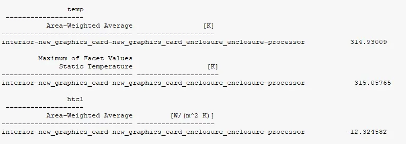
Maximum Temperature attained by the Processor computed is, 315.05 k and there is no much difference from the average temperature 314.93 K

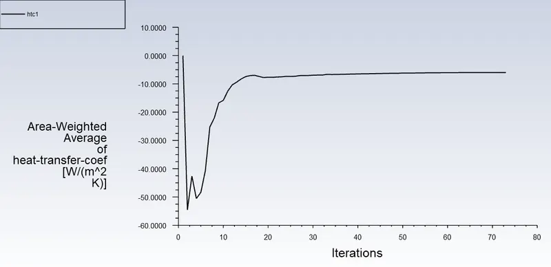
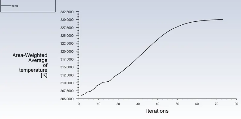
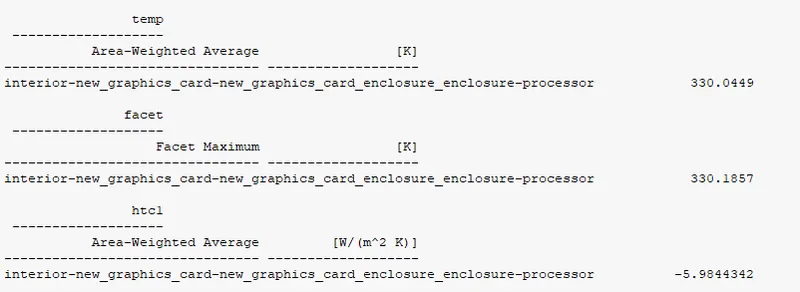
For Refined mesh(1m/s),

Heat Transfer coefficient,

Area weighted Average - Temperature,

Computed values,

	Heat Transfer       coefficient(`W/((m^2)K)`)	Maximum  Temperature(K)	Area weighted Average - Temperature(K)
Coarse mesh(5m/s)	-15.10	313.37	313.35
Refined mesh(5m/s)	-17.76	311.53	311.41
Refined mesh(3m/s)	-12.32	315.05	314.93
Refined mesh(1m/s)	-5.98	330.18	330.04

 Conclusion:

As the number of elements increases the accurate results of temperature distribution is obtained

From the above table, we can conclude that, the net temperature of components of graphics cards decreases with an increase in inlet velocity.

Hence, we can assume that a higher inlet velocity results in better cooling and lower the average temperature thus keeping the components safe from damage.

Furthermore, it can be observed that the temperature of components increases as the inlet velocity decreases from 5 m/s to 1m/s, also proving that higher velocity results in better cooling.