Central differencing method
since we use CDM our grid points look like
 P=N-Q+1 ==> 5-2+1 = 4th order acuurate
As, it is 4th order approx , hence it is 1D we take 2points on left and 2points on right are initiated to find the values of our desired point , and this method continued throughout the domain to obtain mesh elements(FEM) with a spacing distance of (Δx)
our Taylor series eqn will be,
`(del^2u)/(delx^2)`= af(i-2)+bf(i-1)+cf(i)+df(i+1)+ef(i+2) .........(1)
to find (a,b,c,d,e) we are using taylor's table method ,
Taylor series expansion of eqn(1)
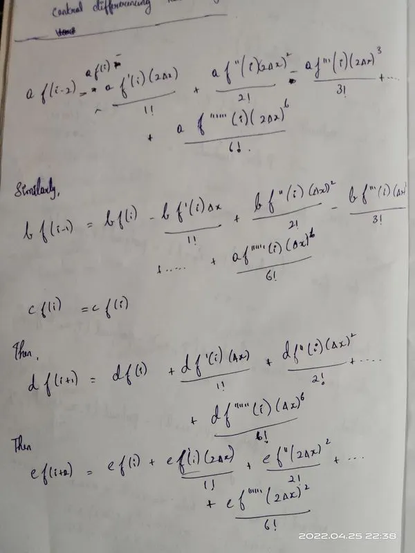
By arranging taylor series expansion in Taylor's table,
| |
f(i) |
Δxf'(i) |
Δx^2 f''(i) |
Δx^3 f'''(i) |
Δx^4f''''(i) |
Δx^5f'''''(i) |
Δx^6f''''''(i) |
| (a)f(i-2) |
a |
-2a |
4a/2 |
-8a/2 |
16a/24 |
-32a/120 |
64a/240 |
| (b)f(i-1) |
b |
-b |
b/2 |
-b/6 |
b/24 |
-b/120 |
b/240 |
| (c)f(i) |
c |
0 |
0 |
0 |
0 |
0 |
0 |
| (d)f(i+1) |
d |
d |
d/2 |
d/6 |
d/24 |
d/120 |
d/240 |
| (e)f(i+2) |
e
|
2e |
4e/2 |
8e/6 |
16e/24 |
-32e/120 |
64e/240 |
|
`sum`(a)f(i-2)+(b)f(i-1)+(c)f(i)+(d)f(i+1)+(e)f(i+2) =
`(del^2u)/ (delx^2)`
|
0 |
0 |
1 |
0 |
0 |
? |
? |
*Note: only for first 5 terms we can assume our hypothesis. That's why we can't say about last 2 terms
Here we have to solve 5eqns to get values of coefficients(a,b,c,d,e)
adding terms in every individual column and that equals to Summation of coefficients.
`A=[[1,1,1,1,1],[ -2, -1, 0 ,1, 2],[2, 1/2, 0, 1/2, 2],[-8/6, -1/6, 0, 1/6, 8/6],[16/24 ,1/24, 0, 1/24, 16/24]]`
`X=[[a],[b],[c],[d],[e]]`
`B=[[0],[0],[1],[0],[0]]`
AX=B
after solving X= inv(A)*B we get,
a=-0.0833
b=1.3333
c=-2.5000
d=1.3333
e=-0.0833
here we can see that a=e ,b=d
Now by dividing both sides of eqn with (`Deltax^2`) , we get
`(del^2u)/(delx^2)= (af(i-2)+bf(i-1)+cf(i)+df(i+1)+ef(i+2))/(Deltax^2)`
By subs values of (a,b,c,d,e) in above eqn we get,
`(del^2u)/(delx^2)= (-0.833333f(i-2)+1.333333f(i-1)-2.500000f(i)+1.333333f(i+1)-0.833333f(i+2))/(Deltax^2)`
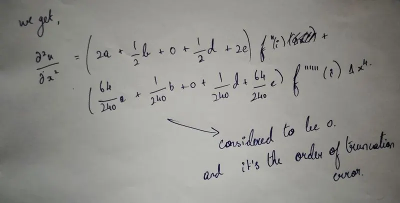
To get the second order derivative the coefficient of f''(i) has to be 1 and other terms are 0
but we haven't assumed anything about f'''''(i)&f''''''(i),
as we know a=e , b=d which makes f''''(i)=0
we have f''(i) & f''''''(i) in our equation
On dividing the eqn with `Deltax^2` , we get
since we know that the order of approx is defined by truncation error term,
we can say that our central differencing scheme is 4th order accurate.
Using Skewed right sided difference
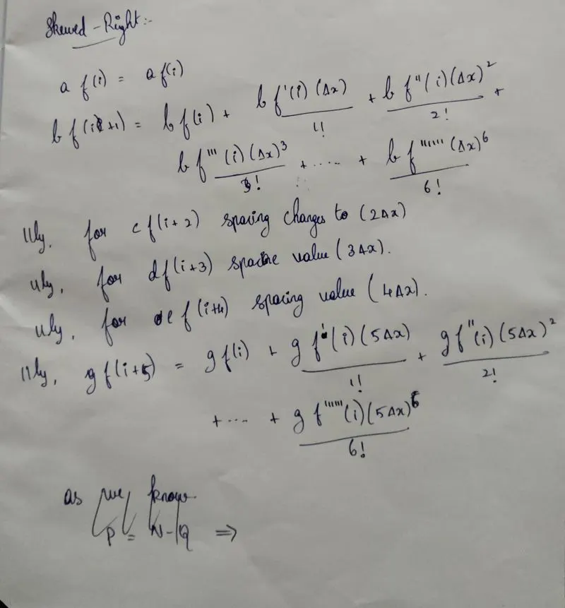
To derive 4th order skewed right at point(i) , we are taking 5points on the right of (i) with an equal spacing of `Delta x`each,

P=N-Q ==>6-2 = 4
`(del^2u)/(delx^2)= (af(i)+bf(i+1)+cf(i+2)+df(i+3)+ef(i+4)+gf(i+5))`
we are using taylor table method to find the coefficients (a,b,c,d,e,g)
By arranging taylor series expansion in taylor table,
| |
f(i) |
`Deltax`f'(i) |
`Deltax^2`f''(i) |
`Deltax^3`f'''(i) |
`Deltax^4`f''''(i) |
`Deltax^5`f'''''(i) |
`Deltax^6`f''''''(i) |
| af(i) |
a |
0 |
0 |
0 |
0 |
0 |
0 |
| bf(i+1) |
b |
b |
b/2 |
b/6 |
b/24 |
b/120 |
b/720 |
| cf(i+2) |
c |
2c |
2c |
8c/6 |
16c/24 |
32c/120 |
64c/720 |
| df(i+3) |
d |
3d |
9d/2 |
27d/6 |
81d/24 |
243d/120 |
729d/720 |
| ef(i+4) |
e |
4e |
8e |
64e/6 |
256e/24 |
1024e/120 |
4096e/720 |
| gf(i+5) |
g |
5g |
25g/2 |
125g/6 |
625g/24 |
3125g/120 |
15625g/720 |
| `(sumaf(i)+bf(i+1)+cf(i+2)+df(i+3)+ef(i+4)+gf(i+5))=((del^2u)/(delx^2))` |
0 |
0 |
1 |
0 |
0 |
0 |
? |
we can assume first 6 terms so that we can't say about last term
we need to get values of coefficients(a,b,c,d,e,g)
adding terms in every individual column and that equals to Summation of coefficients.
A=`[[1, 1, 1, 1, 1, 1],[0, 1, 2, 3, 4, 5],[0, 1/2, 2 ,9/2, 8 ,25/2],[0, 1/6, 8/6, 27/6, 64/6 ,125/6],[0 ,1/24 ,16/24, 81/24, 256/24, 625/24],[ 0 ,1/120, 32/120, 243/120 ,1024/120 ,3125/120]]`
X=`[[a],[b],[c],[d],[e],[g]]`
B=`[[0],[ 0], [1], [0], [0], [0]]`
To get values in X , inv(A)*B is calculated in matlab
a=3.7500
b=-12.8333
c=17.8333
d=-13.0000
e=5.0833
g=-0.8333
Now dividing both eqn by `Deltax^2`
`(del^2u)/(delx^2)= (af(i)+bf(i+1)+cf(i+2)+df(i+3)+ef(i+4)+gf(i+5))/(Deltax^2)`
To get the 2nd order derivative , the coefficient of f''(i) has to be and it is . as well as other terms except f''''''(i) is 0 .
and Now the eqn contains terms of f'(i) & f''''''(i)
we get,
`(del^2 u)/(delx^2)=(0+b/2+(4c)/2+(9d)/2+(16e)/2+(25g)/2)f'' *Deltax^2 +(0+b/720+(64c)/720+(729d)/720+(4096e)/720+(15625g)/720)f'''''' *Deltax^6`
On dividing the eqn by `Deltax^2` ,
`(del^2 u)/(delx^2)=(0+b/2+(4c)/2+(9d)/2+(16e)/2+(25g)/2)f'' +(0+b/720+(64c)/720+(729d)/720+(4096e)/720+(15625g)/720)f'''''' *Deltax^4`
as we discussed before `Deltax^4`denotes Truncation error
Using Skewed Left Sided Difference
To derive 4th order skewed left at point(i) , we are taking 5points on the left of (i) with an equal spacing of `Delta x`each,
P=N-Q ==>6-2 = 4
`(del^2u)/(delx^2)= (af(i-5)+bf(i-4)+cf(i-3)+df(i-2)+ef(i-1)+gf(i))`
we are using taylor table method to find the coefficients (a,b,c,d,e,g)
Taylor series expansion,
`af(i-5)=af(i)-(af'(i)(5Deltax))/(1!)+(af''(i)(5Deltax)^2)/(2!)-(af'''(i)(5Deltax)^3)/(3!)+........+(af''''''(i)(5Deltax)^6)/(6!)`
`bf(i-4)=bf(i)-(bf'(i)(4Deltax))/(1!)+(bf''(i)(4Deltax)^2)/(2!)-(bf'''(i)(4Deltax)^3)/(3!)+........+(bf''''''(i)(4Deltax)^6)/(6!)`
`cf(i-3)=cf(i)-(cf'(i)(3Deltax))/(1!)+(cf''(i)(3Deltax)^2)/(2!)-(cf'''(i)(3Deltax)^3)/(3!)+........+(cf''''''(i)(3Deltax)^6)/(6!)`
`df(i-2)=df(i)-(df'(i)(2Deltax))/(1!)+(df''(i)(2Deltax)^2)/(2!)-(df'''(i)(2Deltax)^3)/(3!)+........+(df''''''(i)(2Deltax)^6)/(6!)`
`ef(i-1)=ef(i)-(ef'(i)(Deltax))/(1!)+(ef''(i)(Deltax)^2)/(2!)-(ef'''(i)(Deltax)^3)/(3!)+........+(ef''''''(i)(Deltax)^6)/(6!)`
gf(i)=gf(i)
By arranging taylor series expansion in taylor table,
| |
f(i) |
`Deltax`f'(i) |
`Deltax^2`f''(i) |
`Deltax^3`f'''(i) |
`Deltax^4`f''''(i) |
`Deltax^5`f'''''(i) |
`Deltax^6`f''''''(i) |
| gf(i) |
g |
0 |
0 |
0 |
0 |
0 |
0 |
| ef(i-11) |
e |
-e |
e/2 |
-e/6 |
e/24 |
-e/120 |
e/720 |
| df(i-2) |
d |
-2d |
2d |
-8d/6 |
16d/24 |
-32d/120 |
64d/720 |
| cf(i-3) |
c |
-3c |
9c/2 |
-27c/6 |
81c/24 |
-243c/120 |
729c/720 |
| bf(i-4) |
b |
-4b |
8b |
-64b/6 |
256b/24 |
-1024b/120 |
4096b/720 |
| af(i-5) |
a |
-5a |
25a/2 |
-125a/6 |
625a/24 |
-3125a/120 |
15625a/720 |
| `(sumgf(i)+ef(i-1)+df(i-2)+cf(i-3)+bf(i-4)+af(i-5))=((del^2u)/(delx^2))` |
0 |
0 |
1 |
0 |
0 |
0 |
? |
coefficients from matlab which is reverse of skewed right ,
g=3.7500
e=-12.8333
d=17.8333
c=-13.0000
b=5.0833
a=-0.8333
Now dividing both eqn by `Deltax^2`
`(del^2u)/(delx^2)= (af(i-5)+bf(i-4)+cf(i-3)+df(i-2)+ef(i-1)+gf(i))/(Deltax^2)`
To get the 2nd order derivative , the coefficient of f''(i) has to be and it is . as well as other terms except f''''''(i) is 0 .
and Now the eqn contains terms of f'(i) & f''''''(i)
we get,
`(del^2 u)/(delx^2)=((25a)/2+8b+(9c)/2+2d+e/2+0)f'' *Deltax^2 +((15625a)/720+(4096b)/720+(729c)/720+(64d)/720+e/720+0)f'''''' *Deltax^6`
On dividing the eqn by `Deltax^2` ,
`(del^2 u)/(delx^2)=((25a)/2+8b+(9c)/2+2d+e/2+0)f'' +((15625a)/720+(4096b)/720+(729c)/720+(64d)/720+e/720+0)f'''''' *Deltax^4`
as we discussed before `Deltax^4`denotes Truncation error
Therefore,we can say that our skewed left sided difference scheme is of 4th order accurate.
Program in matlab for the numerical approximation derived above
we create functions to make the code easier , so functions for central,skewed left, skewed right errors are calculated
functions help us to calculate errors over range of dx , where dx is the spacing btw nodes
saving the function and calling those on main program when need .
Function for CDM
%func for 4th order approx of 2nd order derv using CDM
function error_central_diff = central_differencing(x,dx)
%Analytical func f(x)= exp(x)*cos(x)
analytical_der = -2*exp(x)*sin(x);
%coeff from taylor table calculation p= N-Q+1 -- P= 6-2+1=5
a = -0.0833333333;
b = 1.3333333333;
c = -2.500000;
d = 1.3333333333;
e = -0.0833333333;
%numerical derivative
%central
%diff=((a*f(x-2*dx))+(b*f(x-dx))+(c*f(x))+(d*f(x+dx))+(e*f(x+2*dx)))/ dx^2;
central_differencing_fourth_order_approx =(a*exp(x-2*dx)*cos(x-2*dx)+b*exp(x-dx)*cos(x-dx)+c*exp(x)*cos(x)+d*exp(x+dx)*cos(x+dx)+e*exp(x+2*dx)*cos(x+2*dx))/ dx^2;
error_central_diff = abs(central_differencing_fourth_order_approx - analytical_der);
Function for Skewed right sided difference
%func for 4th order approx of 2nd order derv using CDM
function error_skewed_right = skewed_right(x,dx)
%Analytical ffunc f(x)= exp(x)*cos(x)
analytical_der = -2*exp(x)*sin(x);
%coeff from taylor table calculation p= N-Q+1 -- P= 6-2=4 4th accurate
a = 3.75000;
b = -12.833333333;
c = 17.833333333;
d = -13.00000;
e = 5.083333333;
g = -0.833333333;
%numerical derivative
%skewed_right=((a*f(x))+(b*f(x+dx))+(c*f(x+2*dx))+(d*f(x+3*dx))+(e*f(x+4*dx))+(g*f(x+5*dx)))/ dx^2;
skewed_right_fourth_order_approx =((a*exp(x)*cos(x))+(b*exp(x+dx)*cos(x+dx))+(c*exp(x+2*dx)*cos(x+2*dx))+(d*exp(x+3*dx)*cos(x+3*dx))+(e*exp(x+4*dx)*cos(x+4*dx))+(g*exp(x+5*dx)*cos(x+5*dx)))/ dx^2;
error_skewed_right = abs(skewed_right_fourth_order_approx - analytical_der);
Function for Skewed left sided difference
%func for 4th order approx of 2nd order derv using CDM
function error_skewed_left = skewed_left(x,dx)
%Analytical func f(x)= exp(x)*cos(x)
analytical_der = -2*exp(x)*sin(x);
%coeff from taylor table calculation p= N-Q+1 -- P= 6-2=4 4th accurate
a = -0.8333333333;
b = 5.0833333333;
c = -13.00000;
d = 17.8333333333;
e = -12.8333333333;
g = 3.75000;
%numerical derivative
%skewed_left=((a*f(x-5*dx))+(b*f(x-4*dx))+(c*f(x-3*dx))+(d*f(x-2*dx))+(e*f(x-dx))+(g*f(x)))/ dx^2;
skewed_left_fourth_order_approx =((a*exp(x-5*dx)*cos(x-5*dx))+(b*exp(x-4*dx)*cos(x-4*dx))+(c*exp(x-3*dx)*cos(x-3*dx))+(d*exp(x-2*dx)*cos(x-2*dx))+(e*exp(x-dx)*cos(x-dx))+(g*exp(x)*cos(x)))/ dx^2;
error_skewed_left = abs(skewed_left_fourth_order_approx - analytical_der);
After this step , we are yet to create main program ,
using for loop over a range of dx and using the above functions and
plotting the graph between error vs dx .
Main Program
clear all
close all
clc
x=pi/3;
dx=linspace(pi/4,pi/40000,40);
%creating loop for iteration
for i=1:length(dx)
central_diff_error(i)=central_differencing(x,dx(i));
skewed_right_sided_error(i)=skewed_right(x,dx(i));
skewed_left_sided_error(i)=skewed_left(x,dx(i));
end
%plotting dx vs errors
figure(1)
plot(dx,central_diff_error,'bo-','LineWidth',2)
hold on
grid on
plot(dx,skewed_right_sided_error,'ro-','LineWidth',2)
hold on
plot(dx,skewed_left_sided_error,'go-','LineWidth',2)
xlabel('dx')
ylabel('error')
legend('central diff error','skewed right sided error','skewed left sided error')
figure(2)
loglog(dx,central_diff_error,'bo-','LineWidth',2)
hold on
grid on
loglog(dx,skewed_right_sided_error,'ro-','LineWidth',2)
hold on
loglog(dx,skewed_left_sided_error,'go-','LineWidth',2)
xlabel('dx')
ylabel('error')
legend('central diff error','skewed right sided error','skewed left sided error')
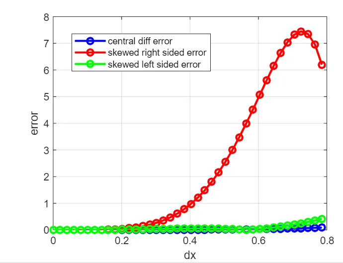
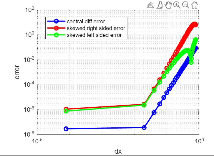
Hence this plot convinces me that I got the desired result , which was shown in assignment help video
By this plot we can conclude that central difference is comparatively more accurate and has lesser error when compared to skewed right and left.
But we cannot use CD in all situations , when it comes to compute numerical approx on boundary , we cannot use CD because CD needs to initialize nodes before and after the boundary so it can't done using this method . In those cases skewed differences plays the role