Week 1- Mixing Tee

MIXING TEE

Objective

• To study the effect of length by comparative analysis of Long Mixing Tee and Short Mixing Tee.
• To discuss the differences that momentum ratio can make.
• To understand that the result obtained is grid independence.
• To compare the mixing effectiveness when hot inlet temperature and the cold inlet temperature, mix together simultaneously with a velocity.

Introduction

In this study, we are going to perform numerical analysis using a software named Ansys Fluent with Boundary conditions .

Ansys Fluent allows to perform major steps in simulation they are pre-processing, solving and post processing.

Mixing tee is device specifically designed with an internal geometry where we can mix two fluid stream into a single fluid stream, hot and cold air with different velocities to mix. Hence we can also find the effect of length in mixing.

Aim

Comparing the mixing effectiveness when hot inlet temperature is 36 degree Celsius and cold inlet is at 19degree Celsius.

Procedure

There are three steps in Numerical analysis. They are,

• Pre-processing (CAD, meshing)
• Solving (setup with boundary conditions)
• Post processing (after calculation- results are illustrated by plots, contours, etc

• Case 1
• Short mixing tee with a hot inlet velocity of 3m/s.
• Momentum ratio of 2, 4.
• Case 2
• Long mixing tee with a hot inlet velocity of 3m/s.
• Momentum ratio of 2, 4.

Momentum ratio = velocity at cold inlet / velocity at hot inlet

Meshing & solver setting

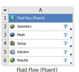
1. Open Ansys workbench --> Right click on geometry--> import short mixing tee part file in spaceclaim.

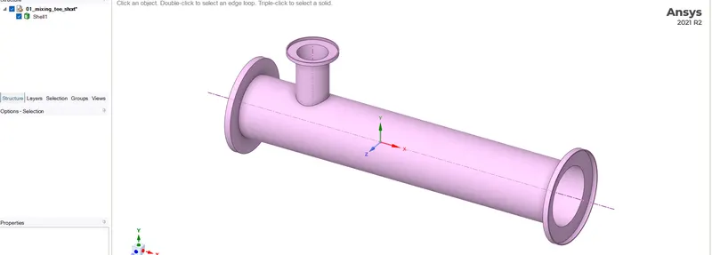
2. Part file will be imported to Space claim.

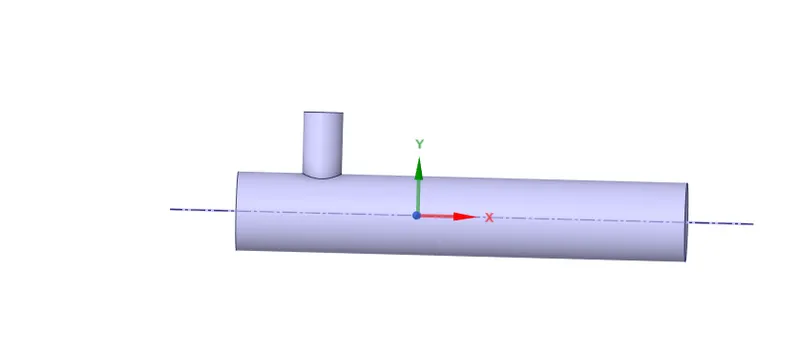
Click on Prepare --> volume extract --> select edges of the part to extract its volume. Then suppress the solid.

3. Going back to the workbench, Click on Mesh. Mesh window appears, Select the faces and name it inlet, outlet, wall using named selection.

--> click on mesh , and enter element size , here we have taken 10mm as element size.

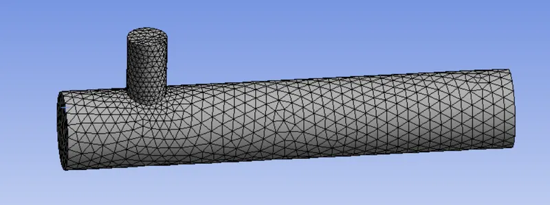
We can also see element quality, from quality option.

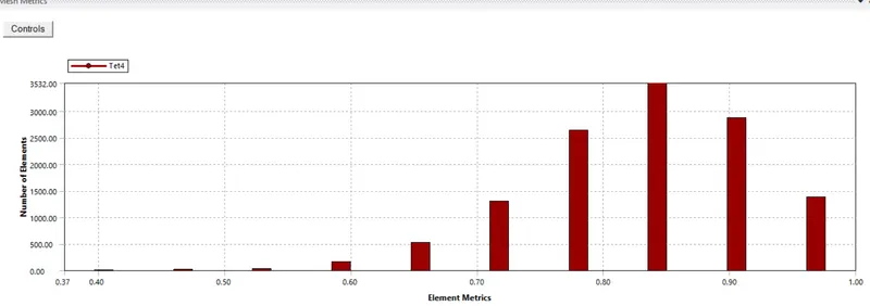
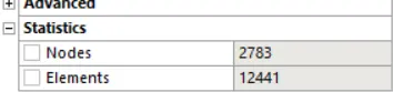
There are 12441 elements after meshing the volume.

Pre-processor and solving

4. After completing mesh, Click on Setup in Ansys workbench.

Fluent window appears

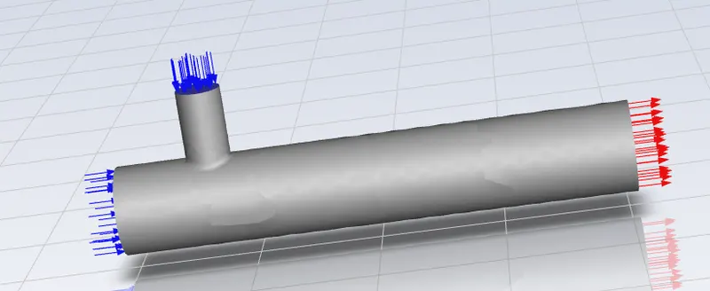
By opening fluent , we have to change our scales and then check mesh , after that select pressure based in setting up physics

In models, select Energy and we are going to compare outputs of k-epsilon and k-omega SST model for the first case and based on our judgment, we use the more suitable model for further cases.

5.Next step is to set up boundary conditions,

- hot inlet velocity of 3m/s with 36 degree Celsius temperature

- as Momentum ratio = velocity at cold inlet / velocity at hot inlet

given Momentum ratio of 2, 4 two different cold velocity , so we have another sub case to solve

cold inlet velocity is 6m/s and 12m/s with 19 degree Celsius temperature.

- outlet condition as pressure outlet and default values.

6. In Solution, Reports --> definition --> more --> area weighted average of temperature at outlet & standard deviation of temperature at outlet.

7. select Hybrid method --> and initialize.

8. After completing Initialization --> Run calculation with no.of.iterations.

9. Results, we can visualize contours and plots respetively, when clicked and selecting what we want to visualize.

Analysis:

1. Case 1
   • Short mixing tee with a hot inlet velocity of 3m/s.
   • Momentum ratio of 2 , which is cold inlet velocity of 6m/s.

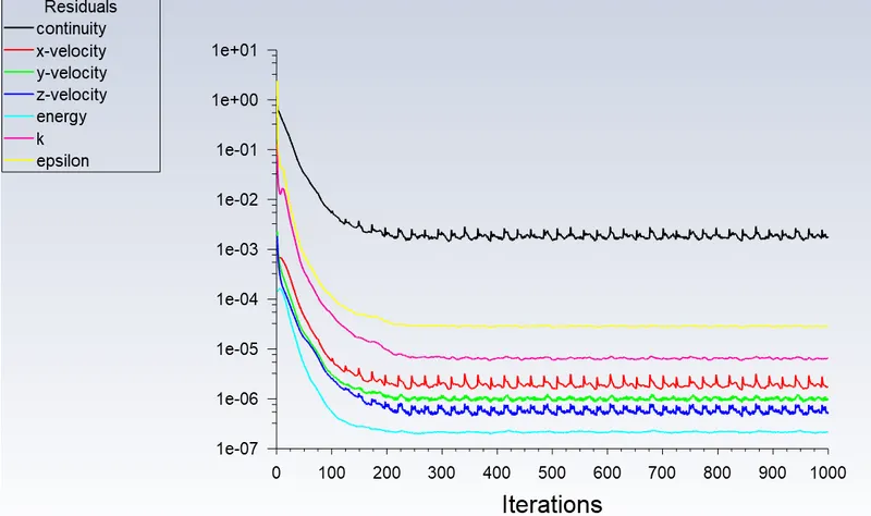
On using k-epsilon: (we have got convergence at 100 iterations)

we get residual plot, standard deviation temperature, area weighted average of temperature.

* Residual plot for K-epsilon model, 6m/s cold inlet velocity :

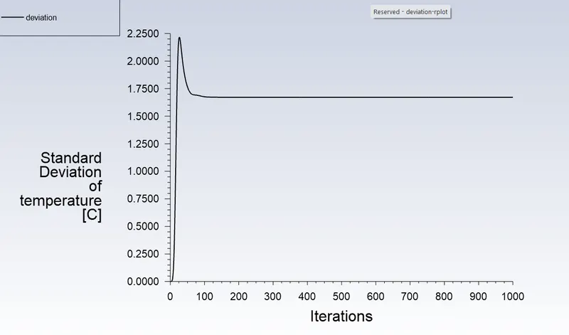
* Standard deviation of temperature for K-epsilon model, 6m/s cold inlet velocity :

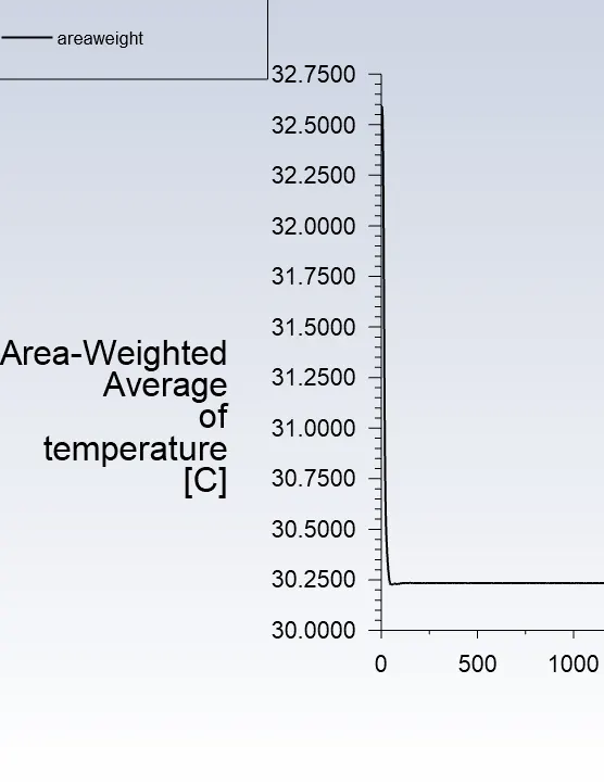
* Area weighted average of temperature for K-epsilon model, 6m/s cold inlet velocity :

*line plots for K-epsilon model, 6m/s cold inlet velocity:

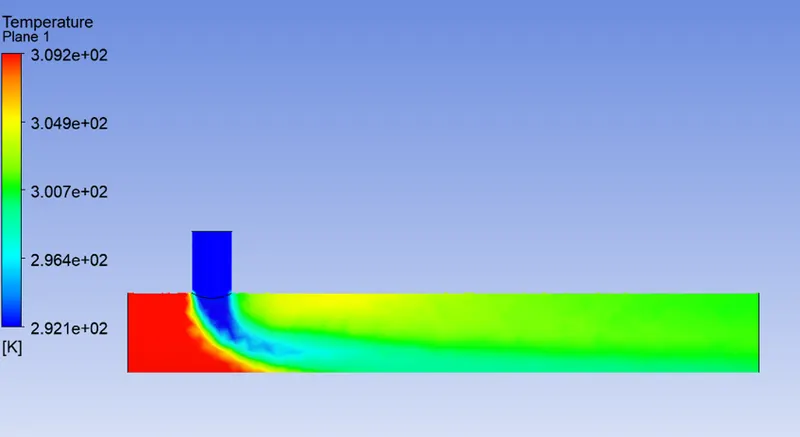
* Contour plot for K-epsilon model, 6m/s cold inlet velocity:

On using k-omega: (we have got convergence after 150 iterations)

we get residual plot, standard deviation temperature, area weighted average of temperature.

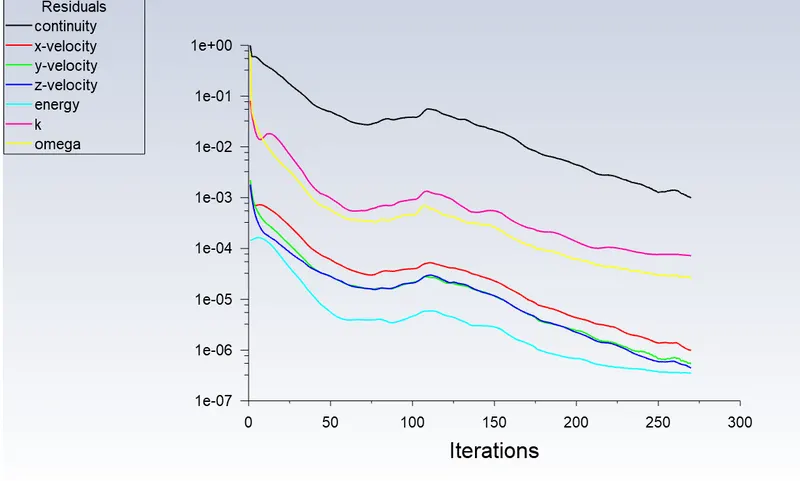
* Residual plot for K-omega model, 6m/s cold inlet velocity :

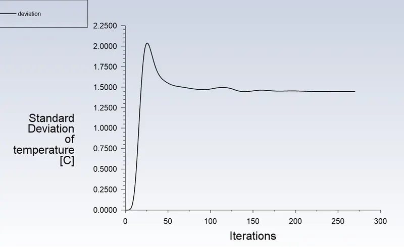
* Standard deviation of temperature for K-omega model, 6m/s cold inlet velocity :

* Area weighted average of temperature for K-omega model, 6m/s cold inlet velocity :

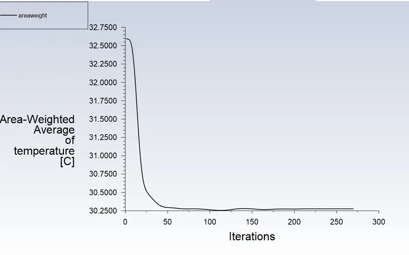
*line plots for K-omega model, 6m/s cold inlet velocity:

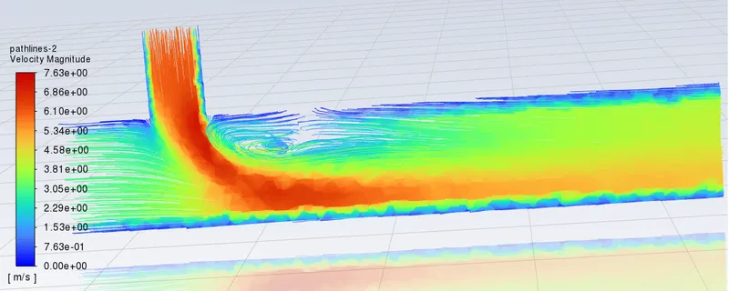
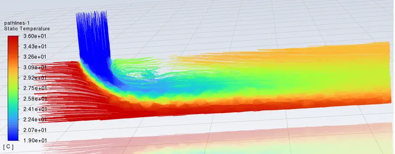
* Contour plot for K-omega model, 6m/s cold inlet velocity:

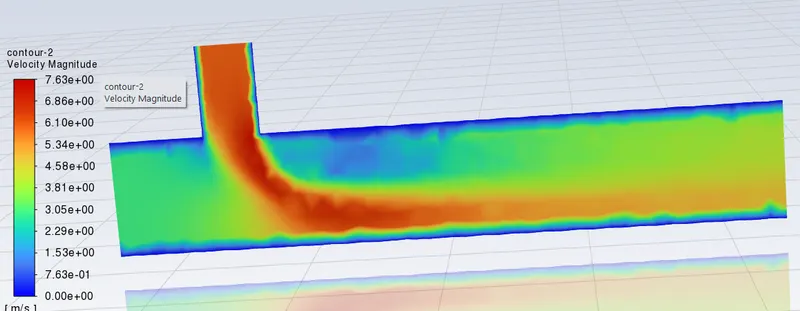
*** Comparatively, K-epsilon takes time and iteration lesser than K-omega, and I don't feel much difference it output too. So I'm choosing K-epsilon for solving this cases.

1. Case 1
   • Short mixing tee with a hot inlet velocity of 3m/s.
   • Momentum ratio of 4 , which is cold inlet velocity of 12m/s.

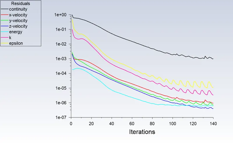
* Residual plot for K-epsilon model, 12m/s cold inlet velocity :

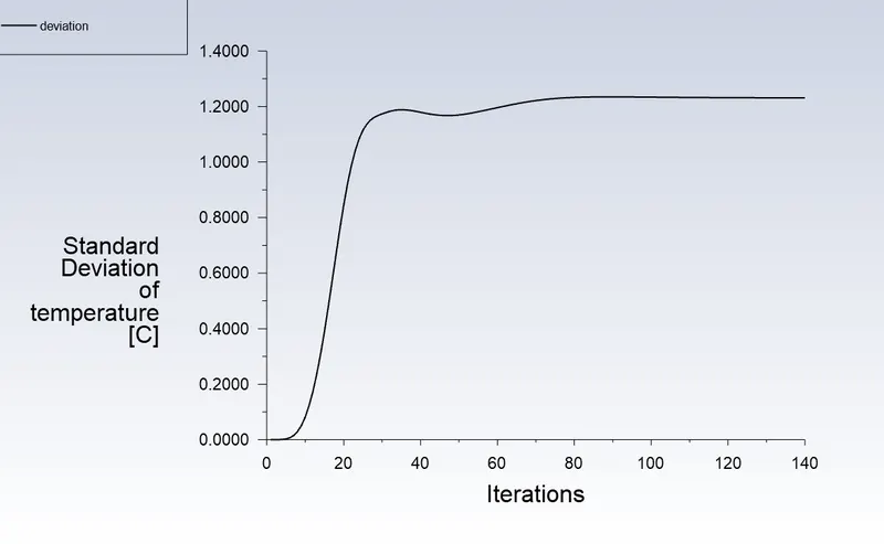
* Standard deviation of temperature for K-epsilon model, 12m/s cold inlet velocity :

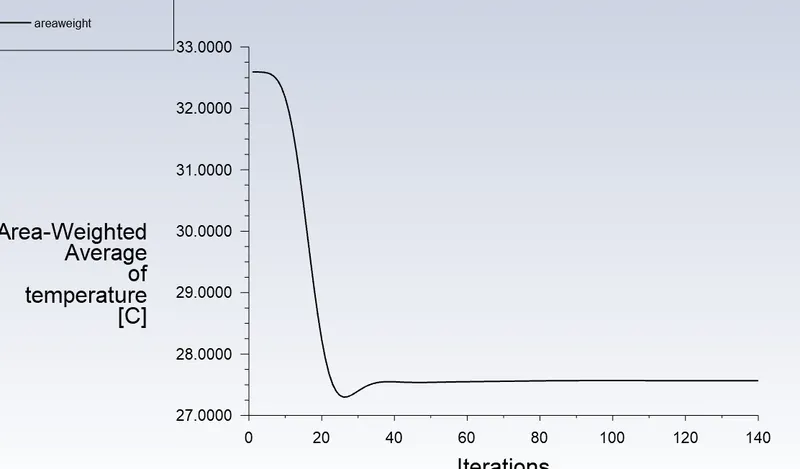
* Area weighted average of temperature for K-epsilon model, 12m/s cold inlet velocity :

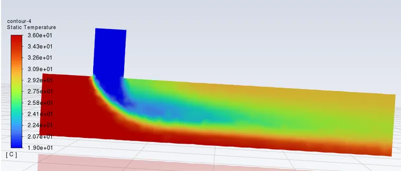
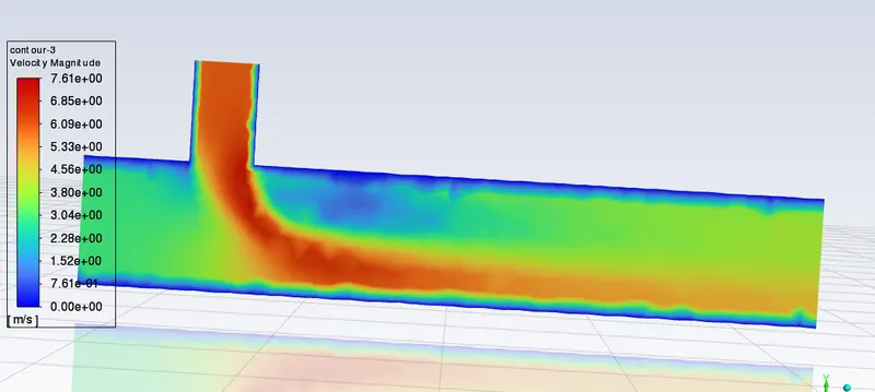
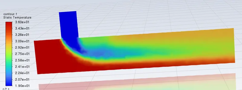
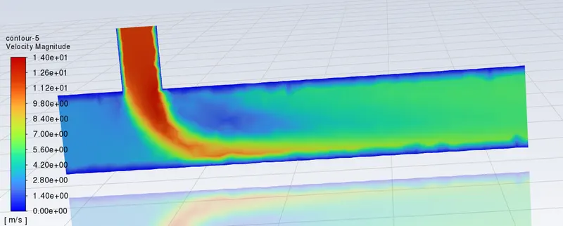
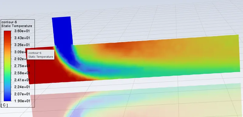
**Contour plot on temperature and velocity:

*

*

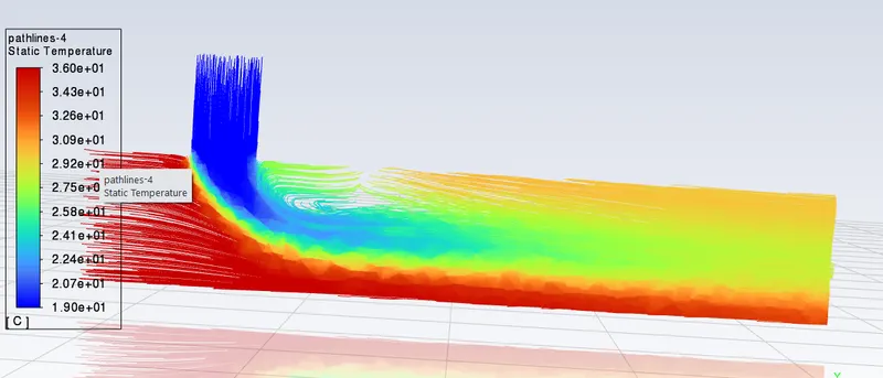
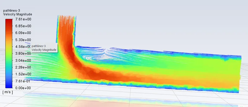
**Pathline plots on Temperature and velocity:

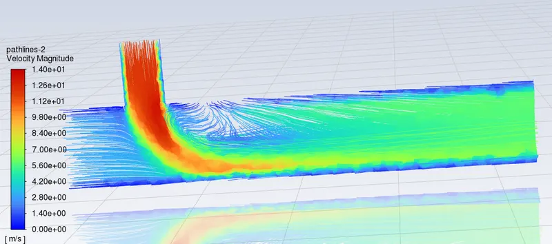
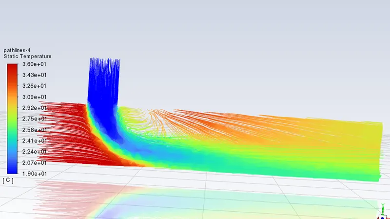
*Finer mesh to perform Mesh independent study:

Mesh with finer elements than before

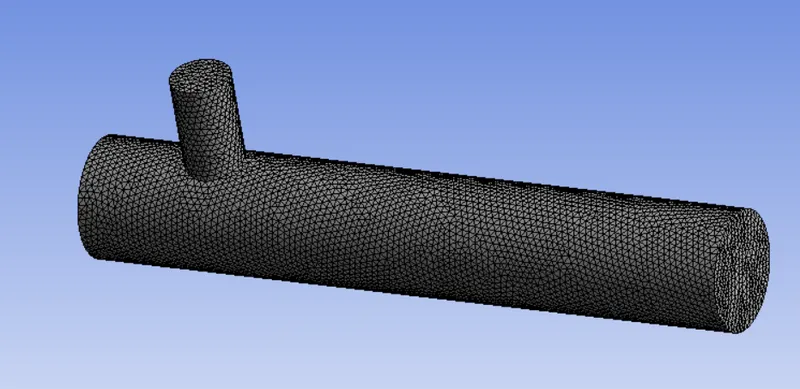
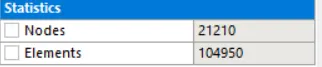
*No.of.elements:

* Area weighted average of temperature for K-epsilon model, 12m/s cold inlet velocity with finer mesh:

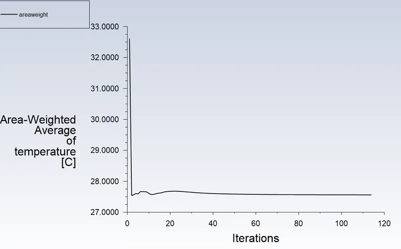
• There isn't any difference of result from finer mesh , Hence the result is Grid Independant.

Case 2 (1)

• Long mixing tee with a hot inlet velocity of 3m/s.
• Momentum ratio of 2 which is cold inlet velocity of 6m/s.

On solving with procedure

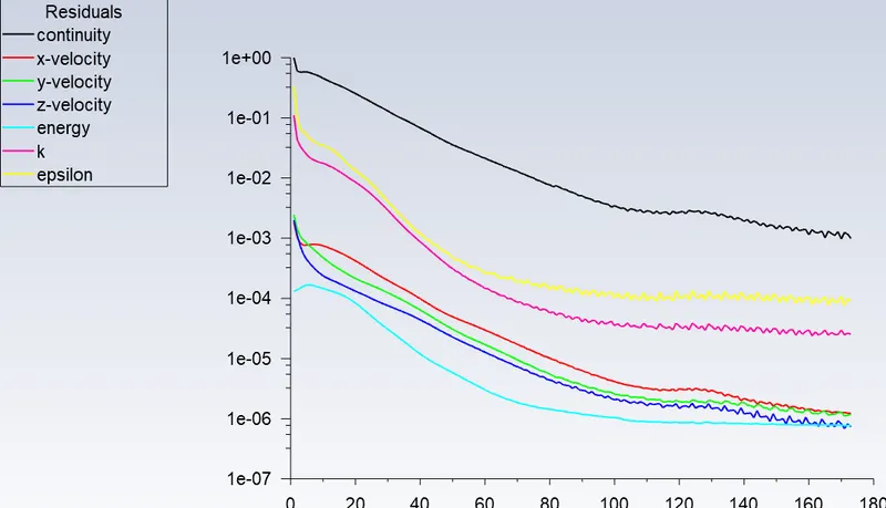
We get residual plot, standard deviation temperature, area weighted average of temperature.

* Residual plot for K-epsilon model, 6m/s cold inlet velocity :

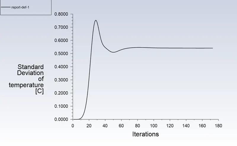
* Standard deviation of temperature for K-epsilon model, 6m/s cold inlet velocity :

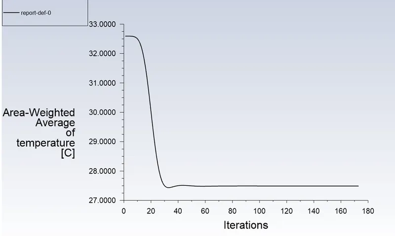
* Area weighted average of temperature for K-epsilon model, 6m/s cold inlet velocity :

*line plots on Temperature and velocity:

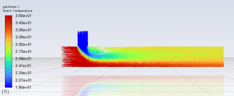
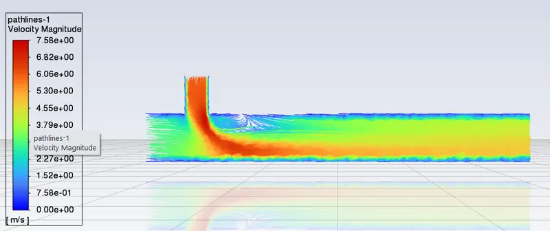
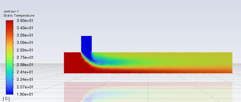
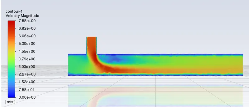
*Contour plots on Temperature and velocity:

Case 2 (2)

• Long mixing tee with a hot inlet velocity of 3m/s.
• Momentum ratio of 4, which is cold inlet velocity of 12m/s.

On solving with procedure

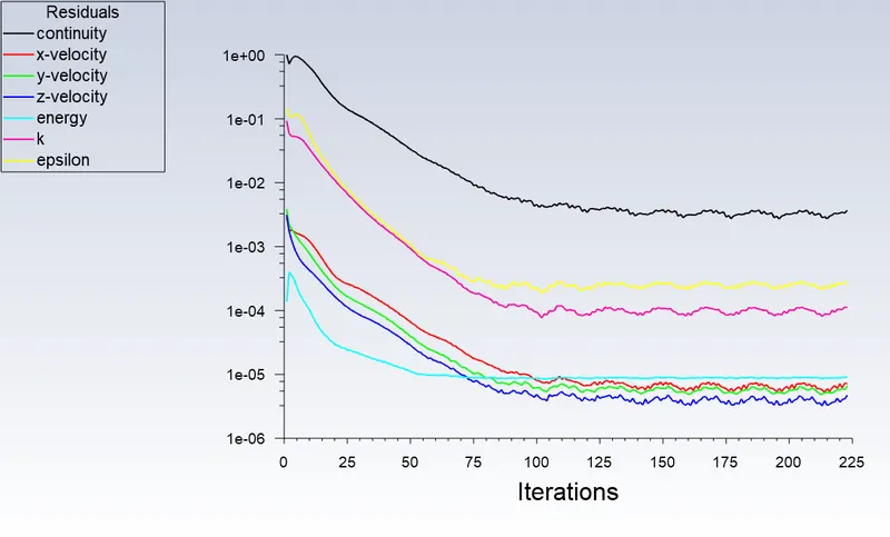
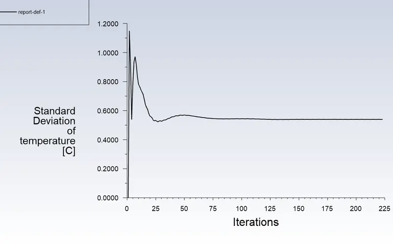
We get residual plot, standard deviation temperature, area weighted average of temperature.

* Residual plot for K-epsilon model, 12m/s cold inlet velocity :

* Standard deviation of temperature for K-epsilon model, 12m/s cold inlet velocity :

* Area weighted average of temperature for K-epsilon model, 12m/s cold inlet velocity :

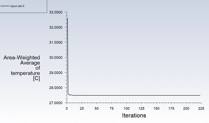
*line plots on Temperature and velocity:

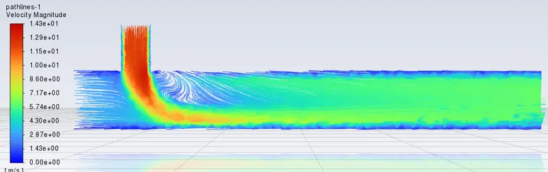
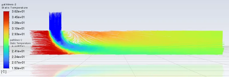
*Contour plots on Temperature and velocity:

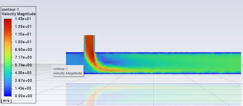
** Table comparing the following values from the 2 cases.

	Short tee 6m/s	Short tee 12m/s	Long tee 6m/s	Long tee 12m/s
Cell count	12441	12441	15540	15540
Average of outlet temperature	30.25	27.5	27.5	27.25
Number of iterations for convergence	100-120	60-80	60-80	30-40

There isn't much difference in decreasing temperature but the effect of length and momentum ratio decreases the iteration counts and when compared there is a slight difference in temperature.

Conclusion:

Hence we conclude simulations with desired result, Area weight average of temperature graph helped me finding average temperature in outlet .

1. Velocity and temperature contour plots on the cut planes along and across the pipe are plotted respectively.
2. Velocity and temperature line plots along and across the length of the pipe are plotted respectively.
3. Performed Mesh independent study for one case and found it is grid independent.
4. Discussed the effect of length and momentum ratio on results, where there is a slight change in temperature and lesser iterations .