Week 5.1 - Mid term project - Solving the steady and unsteady 2D heat conduction problem

OBJECTIVE:

To solve Steady and Unsteady state 2D Heat Conduction Equation by using the point iterative techniques such as Jacobi, Gauss Seidel & Successive over-relaxation for both implicit and explicit schemes using MATLAB.

Problem statement:

1. Computation area is to be a square.
2. Assume nx = ny [No. of points on x-direction is equal to no. of points in y-direction]
3. We assume nx = ny = 10
4. Boundary Conditions are
   Left = 400k
   Right = 600k
   Top = 800k
   Bottom = 900k
5. Apart from the boundary conditions, all other nodes are given an initial temperature of 300k.
6. Various methods to be employed in solving the equation are given below:
   
   
   1. Various States: Steady-state & Unsteady-state Condition
      
   2. Various Schemes: Jacobi, Gauss-seidel & Successive over-relaxation
      
   3. Various Methods to be used in Unsteady-state: IMPLICIT & EXPLICIT

By using Point iterative method, solve the 2D Heat Conduction Equation and plot the Temperature Contour for all the three iterative methods namely Jacobi, Gauss-Siedel & SOR for Steady and Unsteady conditions under IMPLICIT scheme also additionally solving the EXPLICIT scheme for Unsteady Condition.

Types of Heat Conduction schemes

This transfer of Heat energy may occur under two conditions

• Steady-state condition
• Unsteady/Transient state condition

Unsteady state conditions are a precursor to steady state conditions. No system exists initially under steady state conditions. Some time must pass, after heat transfer is initiated, before the system reaches steady state. During that period of transition the system is under unsteady state conditions.

In order to solve the 2D Heat Conduction problem, the governing equations for respective conditions with respect to cartesian coordinates should be discretized to enter that in a code

MATLAB Code:

For Steady state:

%% 2D HEAT CONDUCTION ON A FLAT PLATE

nx = 6;

ny = 6;

Lx = 1;

Ly = 1;

dx = Lx/nx;

dy = Ly/ny;

x = linspace(0,Lx,nx);

y = linspace(0,Ly,ny);

%

% T = meshgrid(x,y)

T = 300*ones(nx,ny);

TL = 400;

TR = 800;

TT = 600;

TB = 900;

T(:,1) = TL;

T(:,end) = TR;

T(1,:) = TT;

T(end,:) = TB;

T(1,1) = 0.5*(TL+TT);

T(1,nx) = 0.5*(TR+TT);

T(ny,1) = 0.5*(TL+TB);

T(nx,ny) = 0.5*(TR+TB);

tol = 1e-4;

error = 1;

error_GS = 1;

% Copy

T_old = T;

T_initial = T;

% JACOBIAN SOLVER

iter = 0;

while(error>tol)

for j = 2:ny-1

for i = 2:nx-1

TL = T_old(i,j-1); TR = T_old(i,j+1); TT = T_old(i-1,j); TB = T_old(i+1,j);

T(i,j) = 0.25*(TL + TR + TT + TB );

end

end

iter = iter+1;

error(iter) = max(max(abs(T-T_old)));

T_old = T;

figure(1)

contourf(flipud(T),'ShowText','ON')

pause(0.03)

xlabel('Xaxis')

ylabel('T')

title(sprintf('Steady State Jacobi iterations = %d',iter));

end

% Re-initialize fields for GS

T_GS = T_initial;

T_old = T_initial;

% GS SOLVER

iter_GS = 0;

while(error_GS>tol)

for j = 2:ny-1

for i = 2:nx-1

TL = T_GS(i,j-1); TR = T_GS(i,j+1); TT = T_GS(i-1,j); TB = T_GS(i+1,j);

T_GS(i,j) = 0.25*(TL + TR + TT + TB );

end

end

iter_GS = iter_GS+1;

error_GS(iter_GS) = max(max(abs(T_GS-T_old)));

T_old = T_GS;

figure(2)

contourf(flipud(T_GS),'ShowText','ON')

pause(0.03)

xlabel('Xaxis')

ylabel('T_GS')

title(sprintf('Steady State GS iterations = %d',iter_GS));

end

% Re-initialize fields for SOR

T_GS = T_initial;

T_SOR = T_initial;

T_old = T_initial;

% SOR SOLVER

iter_SOR = 0;

error_SOR = 1;

r = 0.5

while(error_SOR>tol)

for j = 2:ny-1

for i = 2:nx-1

TL = T_GS(i,j-1); TR = T_GS(i,j+1); TT = T_GS(i-1,j); TB = T_GS(i+1,j);

T_GS(i,j) = 0.25*(TL + TR + TT + TB );

T_SOR(i,j) = (1-r)*T_old(i,j) + r*T_GS(i,j);

end

end

iter_SOR = iter_SOR+1;

error_SOR(iter_SOR) = max(max(abs(T_SOR-T_old)));

T_old = T_SOR;

figure(3)

contourf(flipud(T_SOR),'ShowText','ON')

pause(0.03)

title(sprintf('Steady State SOR iterations = %d',iter_SOR));

end

Output:

IMPLICIT Scheme Unsteady/Transient-state Condition Program:

Unsteady-state Equation discretization:

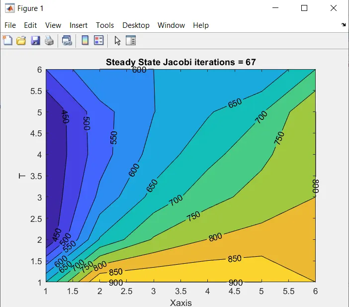
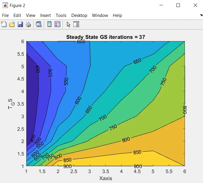
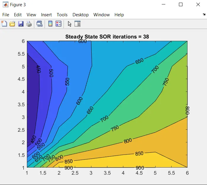
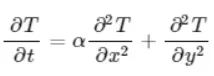
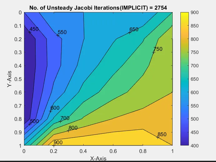
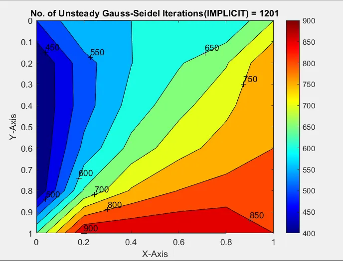
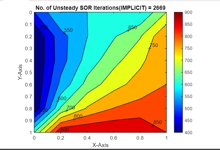
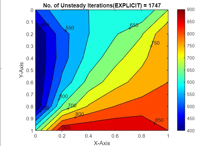
Non-steady-state situations appear after an imposed change in temperature at a boundary as well as inside of an object, as a result of a new source or sink of heat suddenly introduced within an object, causing temperatures near the source or sink to change in time.

MATLAB Code for Unsteady state:

close all

clear all

clc

%Solving the Unsteady state 2D heat conduction by Jacobi Method(IMPLICIT SCHEME)

%Input Parameters

%Number of grid points

nx = 6;

ny = nx;

nt = 1200;

x = linspace(0,1,nx);

y = linspace(0,1,ny);

dx = x(2) - x(1);

dy = dx;

%Absolute error criteria > tolerance

error = 9e9;

tolerance = 1e-4;

dt = 1e-3;

%Defining Boundary conditions

T_L = 400;

T_T = 600;

T_R = 800;

T_B = 900;

T = 300*ones(nx,ny);

T(2:ny - 1, 1) = T_L;

T(2:ny - 1, nx) = T_R;

T(1, 2:nx - 1) = T_T;

T(ny, 2:nx - 1) = T_B;

%Calculating Average temperature at corners

T(1,1) = (T_T + T_L)/2;

T(nx,ny) = (T_R + T_B)/2;

T(1,ny) = (T_T + T_R)/2;

T(nx,1) = (T_L + T_B)/2;

%Assigning orginal values to T

T_old = T;

T_initial = T;

%Calculation of 2D steady heat conduction EQUATION by Successive over-relaxation method

k1 = 1.1*(dt/(dx^2));

k2 = 1.1*(dt/(dy^2));

Jacobi_iteration = 1;

for k = 1:nt

error = 9e9;

while(error > tolerance)

for i = 2:nx - 1

for j = 2:ny - 1

Term_1 = 1/(1 + (2*k1) + (2*k2));

Term_2 = k1*Term_1;

Term_3 = k2*Term_1;

H = (T_old(i-1,j)) + (T_old(i+1,j));

V = (T_old(i,j+1)) + (T_old(i,j-1));

T(i,j) = (T_initial(i,j)*Term_1) + (H*Term_2) + (V*Term_3);

end

end

error = max(max(abs(T_old - T)));

T_old = T;

Jacobi_iteration = Jacobi_iteration + 1;

end

T_initial = T;

%Plotting

figure(1)

contourf(x,y,T)

clabel(contourf(x,y,T))

colorbar

set(gca, 'ydir', 'reverse')

xlabel('X-Axis')

ylabel('Y-Axis')

title(sprintf('No. of Unsteady Jacobi Iterations(IMPLICIT) = %d', Jacobi_iteration));

pause(0.03)

end

%Gauss_Seidel_iteration

%Re-assigning orginal values to T

T_GS = T_initial;

T_old = T_initial;

iter_GS = 1;

for k = 1:nt

error_GS = 9e9;

while(error_GS > tolerance)

for c = 2:nx - 1

for d = 2:ny - 1

Term_1 = 1/(1 + (2*k1) + (2*k2));

Term_2 = k1*Term_1;

Term_3 = k2*Term_1;

H = (T(c-1,d)) + (T_old(c+1,d));

V = (T(c,d+1)) + (T_old(c,d-1));

T(c,d) = (T_GS(c,d)*Term_1) + (H*Term_2) + (V*Term_3);

end

end

error_GS(iter_GS) = max(max(abs(T_old-T_GS)));

T_old = T_GS;

iter_GS = iter_GS + 1;

end

T_GS = T_initial;

%Plotting

figure(2)

contourf(x,y,T_GS)

clabel(contourf(x,y,T_GS))

colorbar

colormap(jet)

set(gca, 'ydir', 'reverse')

xlabel('X-Axis')

ylabel('Y-Axis')

title(sprintf('No. of Unsteady Gauss-Seidel Iterations(IMPLICIT) = %d', iter_GS));

pause(0.03)

end

%%SOR iteration

%Assigning orginal values to T_SOR

T_old = T_initial;

T_SOR = T_initial;

T_end = T_initial;

%Calculation of 2D steady heat conduction EQUATION by Successive over-relaxation method

k1 = 1.1*(dt/(dx^2));

k2 = 1.1*(dt/(dy^2));

iter_SOR = 1;

for k = 1:nt

error = 9e9;

r = 0.6;

while(error > tolerance)

for i = 2:nx - 1

for j = 2:ny - 1

Term_1 = 1/(1 + (2*k1) + (2*k2));

Term_2 = k1*Term_1;

Term_3 = k2*Term_1;

H = (T_SOR(i-1,j)) + (T_old(i+1,j));

V = (T_SOR(i,j+1)) + (T_old(i,j-1));

T_SOR(i,j) = (T_initial(i,j)*Term_1) + (H*Term_2) + (V*Term_3);

T_end(i,j) = ((1-r)*T_old(i,j)) + (T_SOR(i,j)*r);

end

end

error = max(max(abs(T_old - T_SOR)));

T_old = T_end;

iter_SOR = iter_SOR + 1;

end

T_initial = T_end;

%Plotting

figure(3)

contourf(x,y,T_SOR)

clabel(contourf(x,y,T_SOR))

colorbar

colormap(jet)

set(gca, 'ydir', 'reverse')

xlabel('X-Axis')

ylabel('Y-Axis')

title(sprintf('No. of Unsteady SOR Iterations(IMPLICIT) = %d', iter_SOR));

pause(0.03)

end

Output:

EXPLICIT - Unsteady/Transient state Condition Program

close all

clear all

clc

%Solving the Unsteady state 2D heat conduction (EXPLICIT SCHEME)

%Input Parameters

%Number of grid points

nx = 6;

ny = nx;

nt = 1200;

x = linspace(0,1,nx);

y = linspace(0,1,ny);

dx = x(2) - x(1);

dy = dx;

%Absolute error criteria > tolerance

error = 9e9;

tolerance = 1e-4;

dt = 1e-3;

%Defining Boundary conditions

T_L = 400;

T_T = 600;

T_R = 800;

T_B = 900;

T = 300*ones(nx,ny);

T(2:ny - 1, 1) = T_L;

T(2:ny - 1, nx) = T_R;

T(1, 2:nx - 1) = T_T;

T(ny, 2:nx - 1) = T_B;

%Calculating Average temperature at corners

T(1,1) = (T_T + T_L)/2;

T(nx,ny) = (T_R + T_B)/2;

T(1,ny) = (T_T + T_R)/2;

T(nx,1) = (T_L + T_B)/2;

%Assigning orginal values to T

T_initial = T;

T_old = T;

%Calculation of 2D steady heat conduction EQUATION by Successive over-relaxation method

iterative_solver = 1;

k1 = 1.1*(dt/(dx^2));

k2 = 1.1*(dt/(dy^2));

if iterative_solver == 1

Steady_Explicit = 1;

for k = 1:nt

error = 1;

while(error > tolerance)

for i = 2:nx - 1

for j = 2:ny - 1

Term_1 = T_old(i,j);

Term_2 = k1*(T_old(i+1,j) - 2*T_old(i,j) + (T_old(i-1,j)));

Term_3 = k2*(T_old(i,j+1) - 2*T_old(i,j) + T_old(i,j-1));

T(i,j) = Term_1 + Term_2 + Term_3;

end

end

error = max(max(abs(T_old - T)));

T_old = T;

Steady_Explicit = Steady_Explicit + 1;

end

end

end

%Plotting

figure(1)

contourf(x,y,T)

clabel(contourf(x,y,T))

colorbar

colormap(jet)

set(gca, 'ydir', 'reverse')

xlabel('X-Axis')

ylabel('Y-Axis')

title(sprintf('No. of Unsteady Iterations(EXPLICIT) = %d', Steady_Explicit));

pause(0.03);

Output:

CONCLUSIONS:

From the above outputs of various methods & comparing their No. of iterations, we can conclude that

• Jacobi > Gauss-seidel > Successive over-relaxation according to the No. of iterations computed for all methods & Schemes.
  
  
• When comparing Steady state and Unsteady state, it is proven that Steady state is the most successful one as it takes least number of iterations and least time to compute.