Week 8 - Simulation of a backward facing step in OpenFOAM

Simulation of a backward-facing step in OpenFOAM

Aim:-

• Simulate an incompressible-laminar-viscous flow through the backward facing step geometry.
• Perform transient simulation; choose solver based on the described physics of the flow in problem statement.
• Explain simulation process and way of setting up the problem statement in openFOAM and also, explain every changes that have done inside the reference case files obtained from OpenFOAM tutorials.
• Next, preform two case study, firstly, form simulation of the flow without using any grading factor (i.e., GF = 1) . Secondly, simulate the flow with grading factor of 0.2. The cells should be finer near the walls (including the the step wall).

Objective:-

• Open openFoam tutorials and find the the solver to solve incompressible-laminar-viscous flow problem.
• Next step is to copy required file in solver and paste it in OpenFOAM run folder so that the official file of OpenFoam remain untouched.
• Find out block mesh script file to create domain space and provide mesh specification.
• Find ‘controlDict’ file to edit start and end time for simulation.
• In initial folder ‘0’ edit initial parameter for velocity and pressure according to faces of the given domain.
• Use blockMesh command to generate mesh and checkMesh to verify it.
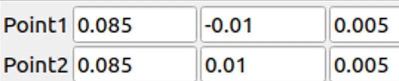
• Open simulation file in paraView and plot the velocity profile at point 0.085m from inlet.
• Repeat above procedure for grading factor 0.2 to check the differences in results.
• Write a detailed report explaining all the command and codes used in project.

Problem Statement:-

simulate an incompressible-laminar-viscous flow through the backward facing step geometry.

perform 2 case studies as described below and compare the results.

Case 1 - Simulate the flow without using any grading factor (i.e., GF = 1)

Case 2 - Simulate the flow with grading factor of 0.2. The cells should be finer near the walls (includig the step wall).

Mesh specification:-

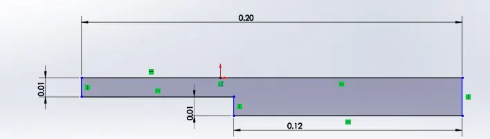
1. Number of cells along the x direction (longer dimension) = 200
2. Number of cells along the longer y direction = 20;

Mesh grading.

Mesh grading is a factor that is,

Grading factor = size of the last cell / size of the first cell

PROCEDURE.

• First, we are creating the run folder in OpenFOAM in which we will be running our simulations.
• And then need to copy the cavity folder to the run folder so that we can make the changes in the blockMeshDict, controlDict, and pressure and velocity files as to run our required simulations, we copying the folder because we are not supposed to make any changes in the original folders in the OpenFOAM.
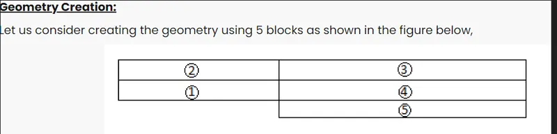
• Then will make the required changes in the blockMeshDict file that is naming the vertices for and then creating the blocks, in this case, there are 21 vertices and 5 blocks while creating blocks we also need to specify the number of mesh points needed along the x, y, and z-direction and also the simple grading should be done along the boundaries.
• then, we need to assign the boundary conditions here, we need to define all the faces in OpenFOAM refers to patches and giving them type that is the inlet and outlet will be the faces (type patch), for top and bottom which are the boundary conditions in this case type will be wall type and setting up these will constitute a particular boundary, then will save these changes in the blockMeshDict.
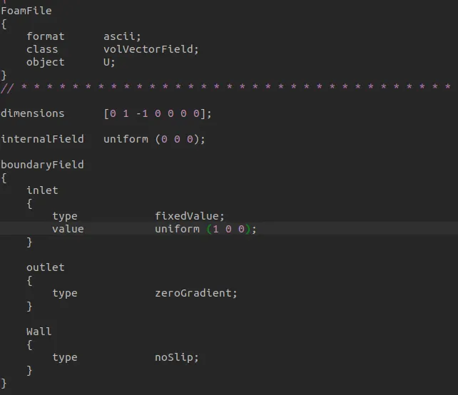
• Then, in the velocity and pressure files, we have to give the value of the velocity at the inlet type will be fixed value here we should assign some value as initial velocity and pressure will be zerogradient and at the outlet velocity type will be zerogradient and pressure will be type fixedvalue that value will be uniform 0, then at front and back velocity type empty and pressure, as well as type empty at the no slip boundaries that is top and bottom velocity, will be type noslip and pressure type empty. And in the transportProperties we can change the nu value in order to obtain the lower courant number.
• And in the controlDict file the simulation time and the time step need be assigned in the way that the courant number should be less than 0.5.
• and then creating the block mesh and then run the simulation using the respective solver after the completion of simulation open the paraview in the paraFoam and plot the velocity profile for the given value.

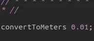
we set units in meter, by converting all type of length in to meter.

Vertices:-

Afterward, in codes, we provide list of vertices by providing x,y,and z coordinates locations; its always start from vertex (0,0,0). so we have to create following geometry.

'

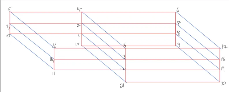
vertices points are,

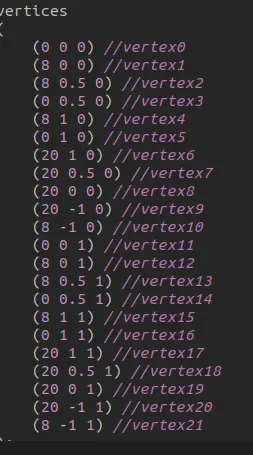these are vertices of backwardstep coded on blockMeshDict file

Mesh generation without any grading factor

In the same blockMesh file go to the lines where we the word hex can be found. That is the line where we specify the faces of the blocks and also the number of cells in X, Y and Z direction.

Next, we are going to define block for meshing. If we look at he mesh format first letter, in block parenthesis, is ‘hex’ which define type of mesh which is hexahedral mesh.

Then, again in parenthesis, we provide vertices number according to order which follow right hand thumb rule, meaning, thumb is the z axis and order of vertices follow rotational order of our other finger.

Then comes, number of mesh grid that we want to divide along x, y, and z length. We define it as (nx,ny,nz) format.

Given mesh specification:

1. Number of cells along the x direction(longer dimension) = 200
2. Number of cells along the longer y direction = 20

Lastly, we give simple grading which is cell expansion ratios

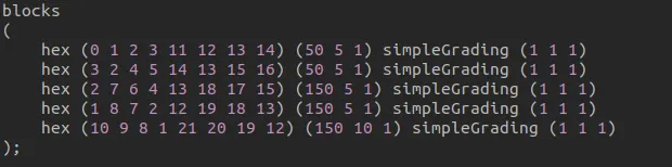
Also we specify the faces as the inlet, outlet and walls

Defining the Boundary Conditions;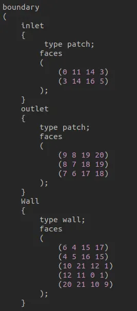

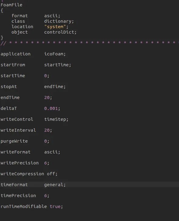
The next step is to navigate to the controlDict folder and specify the simulation time as 20 seconds with dt of 1e-2.The script file looks as follows.

After, editing of blockMeshDic file save it and close it.

Furthermore, we are going to edit ‘controlDict’ file to provides time limits - start time and end time. Also to represent deltat. While selection of deltat CFL value shoud be less than 1. otherwise, the solution could stopped forcibly or it may diverge at the time of converging. So make following changes in ‘controlDict’ file.

Initial setting for Velocity

Initial setting for Pressure:

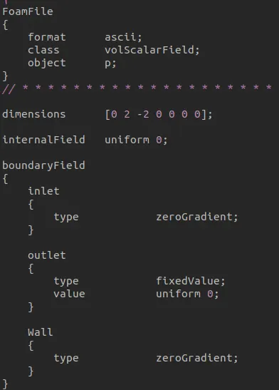
At this point, our problem statement is set, we can now proceed to deploy mesh using ‘blockMesh’ command

Mesh grid:

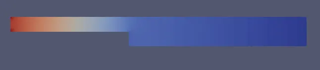
Velocity Distribution along the domain area:-

Pressure Distribution along the domain area:-

Graph (line parameters):

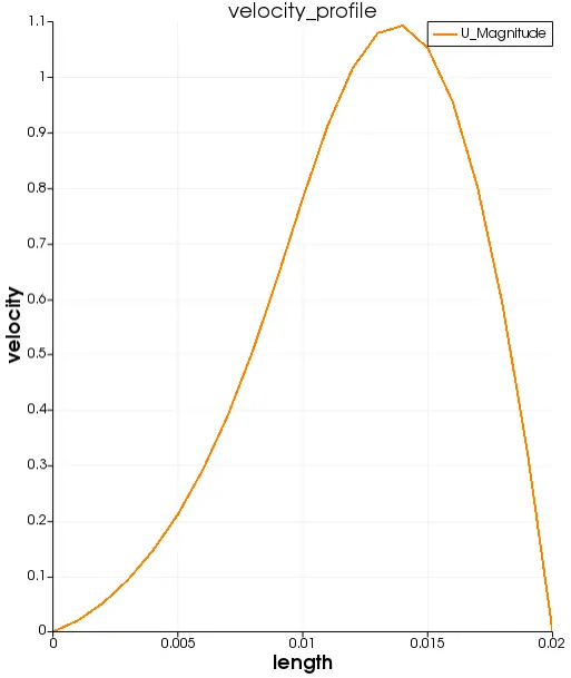
Velocity Plot:-

With Grading Factor 0.2 (cell near All walls)

blockMeshDict is edited in the simple grading of blocks part,

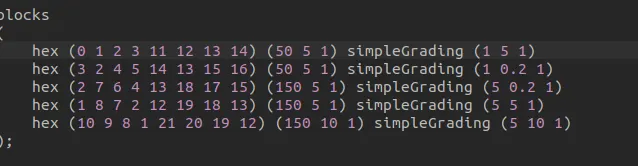
Next,use grading factor 0.2 for all walls in the system.

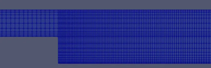
finer mesh near walls,

Velocity Distribution along the domain area:-

Pressure Distribution along the domain area:-

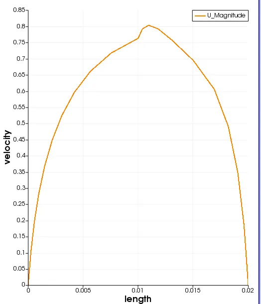
Velocity Plot:-

Results

- Up to this point, we have done plotting velocity plot for both, without grading factor and with 0.2 grading factor, cases. If we take a look at all the three line graph, we can see, the plot for velocity without grading factor seems more smooth and accurate than other two plot. So one can say, grading can disrupt out result. But it is incorrect. Because, if we take good look at it, we can notice, the mesh is fine at step wall along the X-axis but very coarse along Y-axis. Therefore, we are not getting smooth plot for velocity at 0.085 point at Y-axis.

- To understand this thing clearly, we can see below figure, where we can see- on the left side there is coarse mesh and on the right side fine mesh. Above picture, there respective graphs are presented, which can really convince anyone how at any given point mesh produce a plot. The one on the right side mesh is giving very smooth plot except one small pick near point 0.01 and on the other hand, for coarse structured mesh, the curve of graph the curve is not smooth, there are sharp corner forming at the top of the curve.

- After learning how mesh actually works, we should use fine mesh near the point where we expect our results. In CFD fluid always shows large changes near walls and obstacles along its way and to capture those changes effectively we should always use grading or finer mesh near a wall.

- To get effective and reliable results, one should know where to use finer grading factor. In a bid to obtain more effective results, suppose, if we use large number of fine elements, it could use our computation time and also require large computational memory(RAM). Therefore, use of grading is important, so that, we can use fine mesh to capture the flow at boundary wall and obstacles, course mesh at more open area.

- Use fine mesh in the area where maximum chnges happen in velocity, pressure or other property of fluid, to capture more detailed and accurate results.