Week 6 - CHT Analysis on a Graphics card

Aim:- Perform a steady-state conjugate heat transfer analysis on a model of a graphics card.

Objectives:

1. Run the simulation by varying the velocity from 1m/sec to 5m/sec for at least 3 velocities and discuss the results.
2. Find out the maximum temperature and heat transfer coefficient attained by the processor.
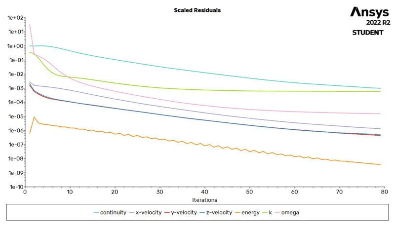
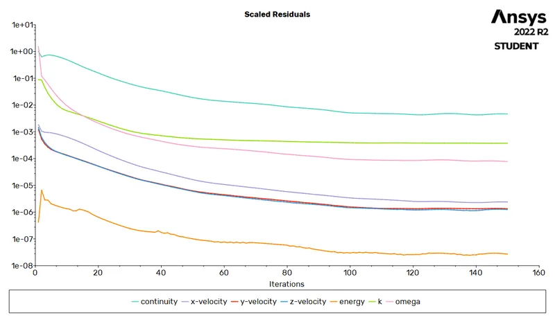
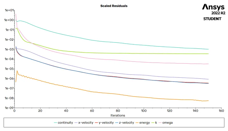
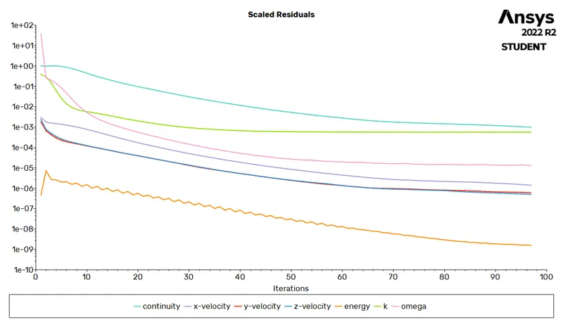
3. Prove that the simulation has achieved convergence with appropriate images and plots.
4. Identify potential hotspots on the model.

Theory:-

Conjugate Heat transfer analysis:- A CHT (Conjugate Heat Transfer) analysis is useful where there are multiple modes of heat transfer in our computational domain, like conduction and convection. Having such a great number of applications for this type of simulation makes it important to be studied in depth.

The Conjugate Heat Transfer (CHT) analysis type allows for the simulation of heat transfer between solid and fluid domains by exchanging thermal energy at the interfaces between them. Typical applications of this analysis type exist as, but are not limited to, the simulation of heat exchangers, cooling of electronic equipment, and general-purpose cooling and heating systems.

we need to enable energy equationand provide the appropiate boundary condition to understand it properly.

Some applications are

• Temperature distribution analysis.
• Heat flux rate analysis – calculation of wall heat flux rates or heat transfer coefficients.
• Visualisation of heat transfer features for improved understanding of system flow phenomena.
• Identification of localised ‘hot spots’ or heat sinks in checking against specified requirements.
• Evaluating variation in temperature peaks for different operating conditions/ failure modes.
• Assessing insulation or heat shield effectiveness and optimising of material selections.
• Coupling CHT with FE analysis to evaluate thermally induced stresses, expansion or fatigue.
• Temperature field analysis
• CFD thermal analysis
• Heat transfer coefficient analysis
• Heat transfer rate analysis

Fundamentals related with heat transfer.

Mode of heat transfer are

1. conuction

2. convection

3. radiation

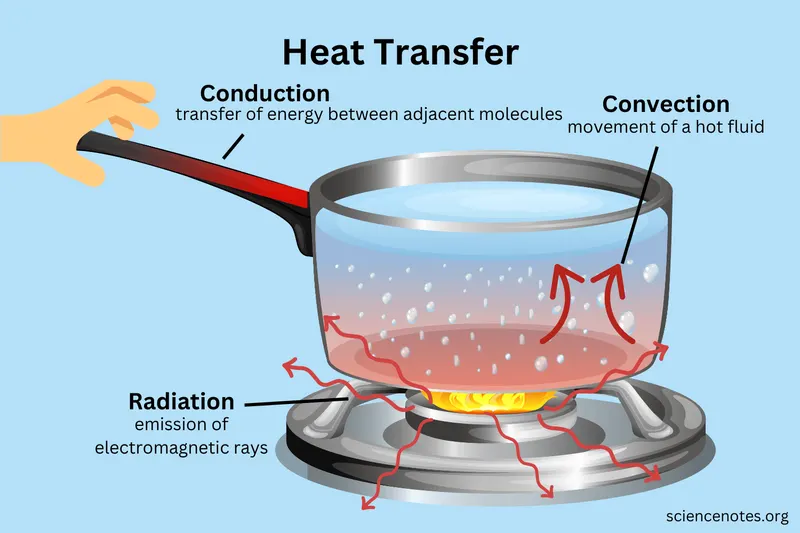
Conduction:- In conduction mode of het transfer the transfer is take place between adjacent molecules, bulk motion is not needed for heat transfer.

this can be calculated using fourier law.

for a plane layer, heat conduction layer for a plane layer is directly proportional to temprature difference and area across the layer but inversely proportional to the layer thickness

this can be governed by

Qc = -k A dt/dx

k is the thermal conductivity( unit Watt/m.k, it is a material property)

A is the area

dt is the temprature difference between the plane

dx is the thickness

Convection:- In convection mode of het transfer the transfer due to fluid flow, bulk motion is needed for heat transfer.

this can be calculated using newtons law.

heat convection directly proportional to temprature difference and area across

Qc = h A dt

h is the convective heat transfer( unit Watt/m^2.k)

A is the normal surface area

dt is the temprature difference between the plane

Radiation: Stefan Boltzman law of radiation

it state that radiation energy emitted from the surface of a black body is directly proportional to the 4th power of absolute temprature

Qr = sigma*T^4

sigma is stefan boltzman constant 5.67*10^-8 Watt/m^2k

Thermal diffusivity: is the ability of the material by which heat can propogate within the material

it is the ratio of thermal conductivity/Rho*c

here rho is the density (kg/m^3)

c is the specific heat (J/kg K)

Nusselt Number: Nusselt no is the ration of convective heat transfer to the conductive heat transfer

convective heat transfer/conductive heat transfer

hl/k

CFD:-Computational fluid dynamics or CFD is the analysis of systems involving fluid flow, heat transfer and associated phenomena such as chemical reactions by means of computer-based simulation.

Practical application in current scenario

• aerodynamics of aircraft and vehicles: lift and drag
  • hydrodynamics of ships
  • power plant: combustion in internal combustion engines and gas
  turbines
  • turbomachinery: flows inside rotating passages, diffusers etc.
  • electrical and electronic engineering: cooling of equipment including
  microcircuits
  • chemical process engineering: mixing and separation, polymer moulding
  • external and internal environment of buildings: wind loading and
  heating/ventilation
  • marine engineering: loads on off-shore structures
  • environmental engineering: distribution of pollutants and effluents
  • hydrology and oceanography: flows in rivers, estuaries, oceans
  • meteorology: weather prediction
  • biomedical engineering: blood flows through arteries and veins

CFD Work Flow:- CFD codes are structured around the numerical algorithms that can tackle fluid flow problems. In order to provide easy access to their solving power all commercial CFD packages include sophisticated user interfaces to input problem parameters and to examine the results

Its threee step process
(i) a pre-processor

involves defination of geometry, grid generation, selection of phenomenon that need to model

(ii) a solver

intergration of governing equation, discretisation and solution

(iii) a post-processor

ploting of contour, graphs and making movies.

In solving fluid flow problems we need to be aware that the underlyingphysics is complex and the results generated by a CFD code are at best asgood as the physics (and chemistry) embedded in it and at worst as good asits operator with CFD

Solving and Modeling Approch:-

There are no way present to understand and analyse the effeciveness of the mixiing tee model.

1. analytical approch

2. simulation approch

3. experimental approch

using analytical approch and experimental approch is time consuming and high cost senario. this could be eliminated by using simulation approch in which we can analyse the system with the actual codition we are intrested in.

To do this we are using ansys fluent solver

we are using fluid flow analysis using Fluent solver because we are interested in the total effectiveness of the fluid in the mechnical tee model, here we are using two different models to analyse the effectiveness of the mixing of fluid.

Approch we are using.

1. We need to open Ansys workbench

2. Choose the Appropiate Solver

3. Assign Appropiate name

4. Choose geometry and select new spaceclaim model.

5. Load the appropiate file

6. Implement the geometrical operation

7. Apply the mesh and provide name selection

8. Choose setup, select the appropiate model

9. Initalisation and running the simulation

10. Result making i.e. countour plots graphs

1. Opening Ansys workbench

2. Choose the Appropiate Solver

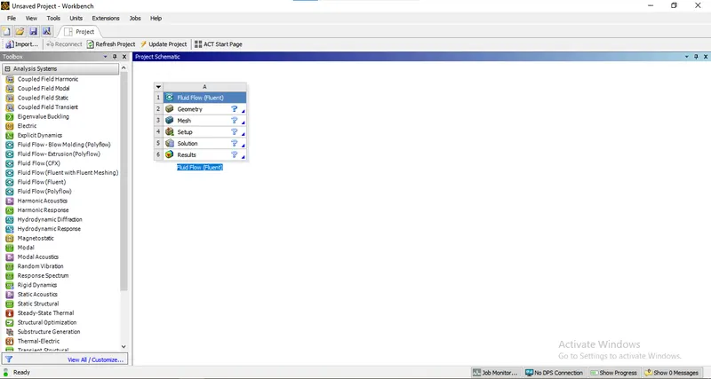
3. Assign Appropiate name

4. Opening of space claim geometry do to geometrical operation

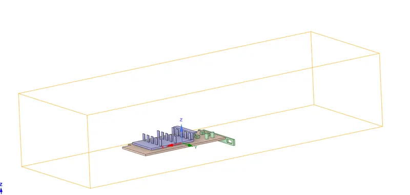
now go to workbench and use share topology

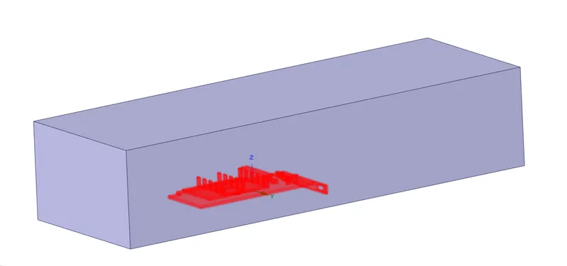
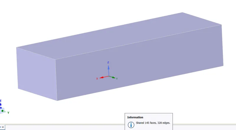
Now we can move to mesh mode

Meshing

Component Name	Fine mesh	Coarse mesh
Processor	.5 mm	1 mm
Fins	1.5 mm	2.5 mm
PCB	.5 mm	1 mm
Enclosure	8 mm	10 mm

Case

Case 1. Fine mesh with U = 3m/s

Case 2. Coarse mesh with U = 3m/s

Case 3. Fine mesh with U = 1m/s

Case 4. Coarse mesh with U = 1m/s

Case 5. Fine mesh with U = 5m/s

Case 6. Coarse mesh with U = 5m/s

Now provide the name selection

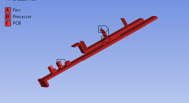
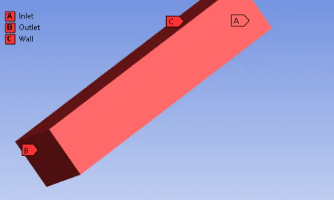
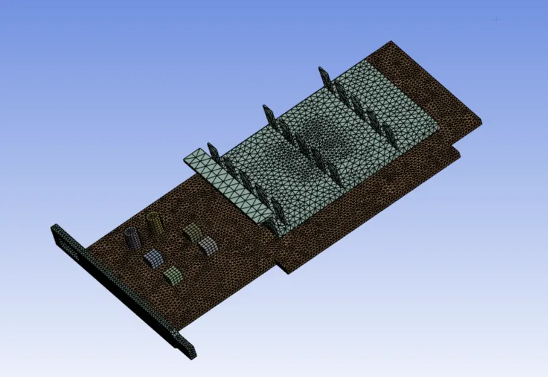
now we done with meshing part move to setup mode

Setup:-

Settings

Solver	Steady state
Energy Equation	ON
Model	Laminar
Inlet	Inlet Velocity
Outlet	Pressure Outlet
Material_(Fluid)	Air, 3 user defined
Cell Zone Condition	Air, 3user defined

Material Property that used for this particular simulation

Material Name	Density(kg/m^3)	Cp(J/kgK)	Thermal Conductivity (W/m.K)
Alluminium	2719	871	202.4
Silicon	2330	703	153
Pcb	55	1210	.027

GO to cell zone and provide the materials to the different components

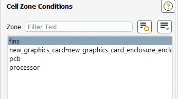
select the component and choose the appropiate material.

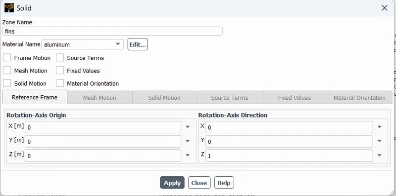
in similar manner we assign the materials to remaining components.

No Create the required reports and countour we are looking for

Results

1. Residuals

for Fine mesh

Fine mesh with U = 5m/s	Fine mesh with U = 3m/s	Fine mesh with U = 1m/s

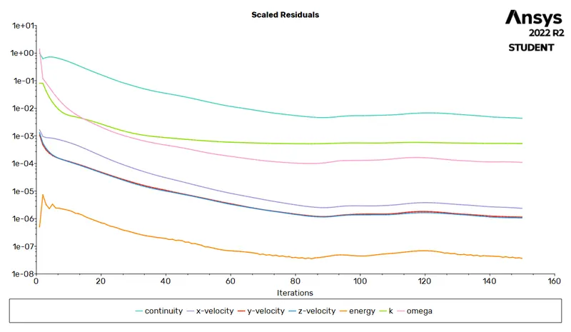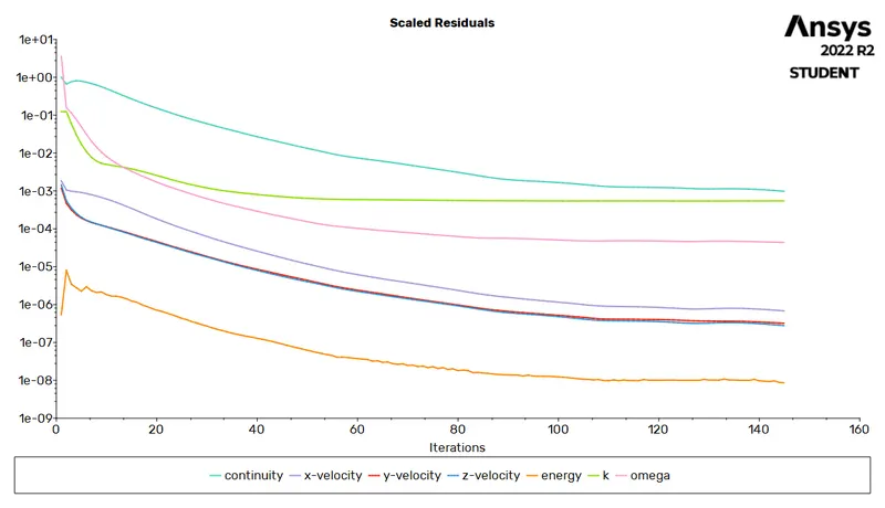for Coarse mesh

Coarse mesh with U = 5m/s	Coarse mesh with U = 3m/s	Coarse mesh with U = 1m/s

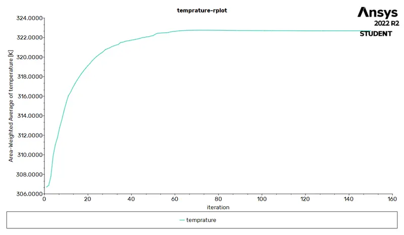
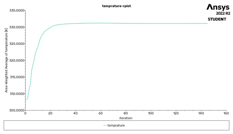
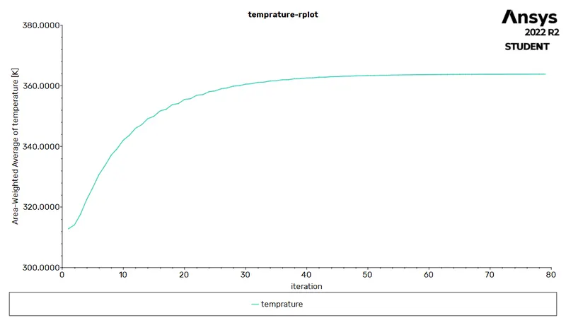
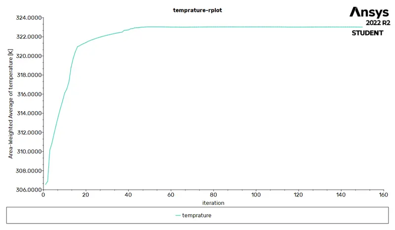
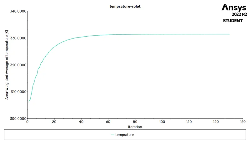
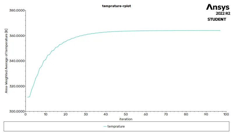
2.Temprature at Processor

for Fine mesh

Fine mesh with U = 5m/s	Fine mesh with U = 3m/s	Fine mesh with U = 1m/s

for Coarse mesh

Coarse mesh with U = 5m/s	Coarse mesh with U = 3m/s	Coarse mesh with U = 1m/s

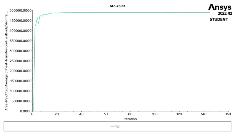
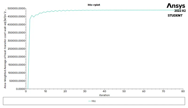
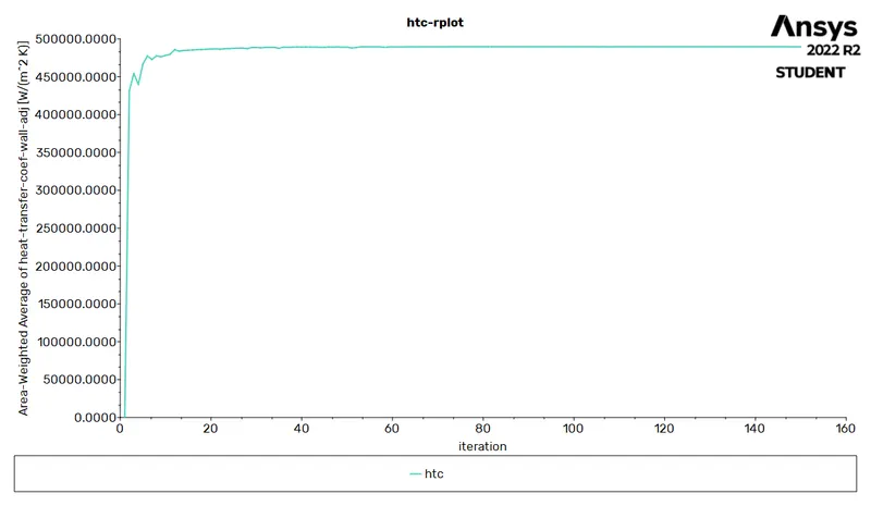
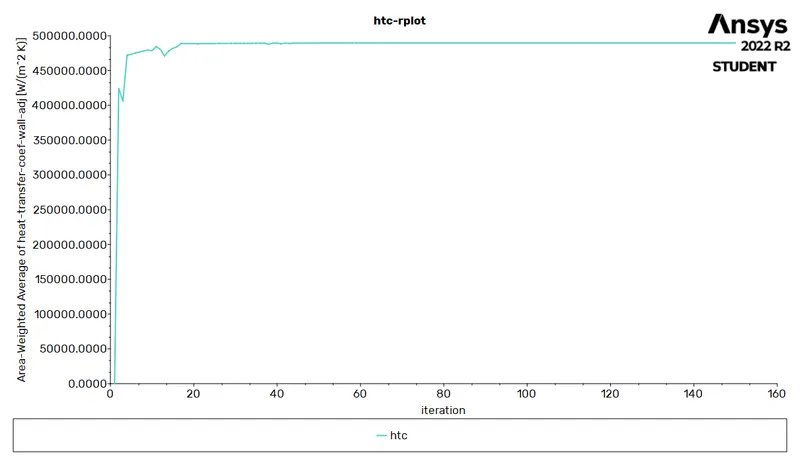
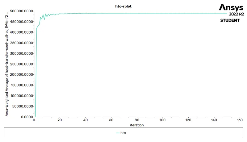
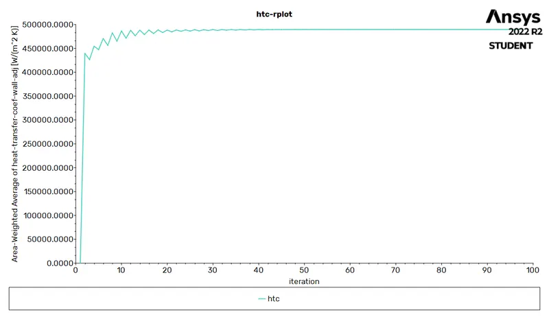
3.HTC

for Fine mesh

Fine mesh with U = 5m/s	Fine mesh with U = 3m/s	Fine mesh with U = 1m/s

for Coarse mesh

Coarse mesh with U = 5m/s	Coarse mesh with U = 3m/s	Coarse mesh with U = 1m/s

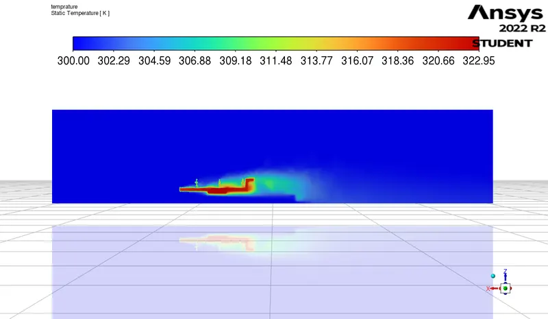
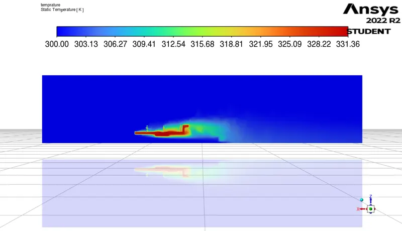
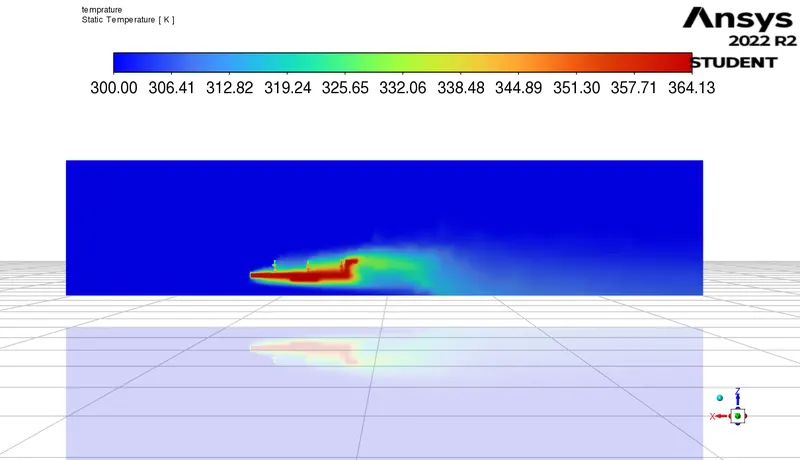
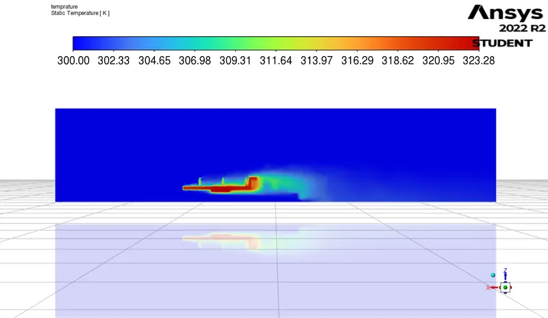
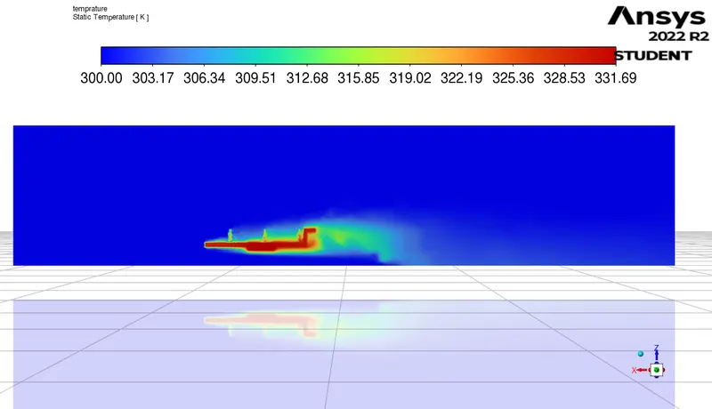
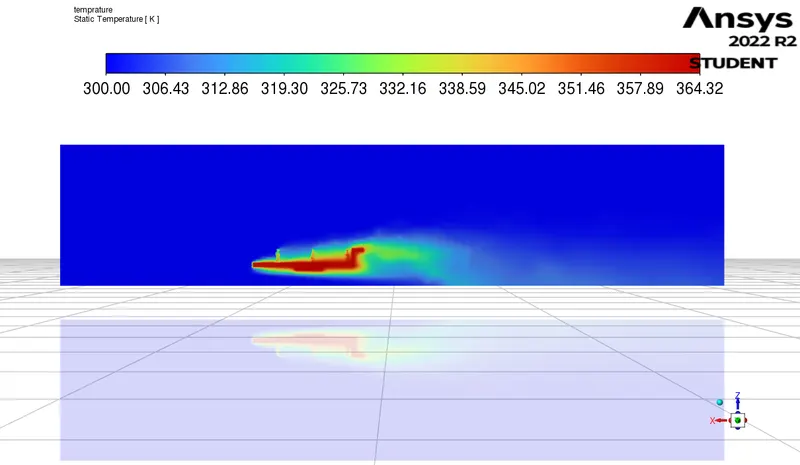
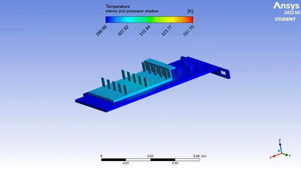
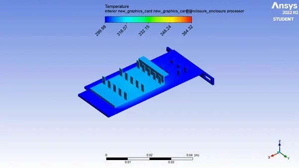
4.Temprature Contour

for Fine mesh

Fine mesh with U = 5m/s	Fine mesh with U = 3m/s	Fine mesh with U = 1m/s

for Coarse mesh

Coarse mesh with U = 5m/s	Coarse mesh with U = 3m/s	Coarse mesh with U = 1m/s

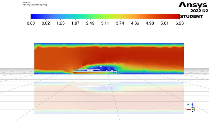
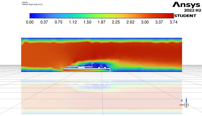
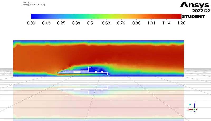
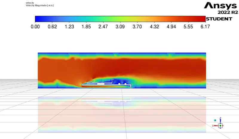
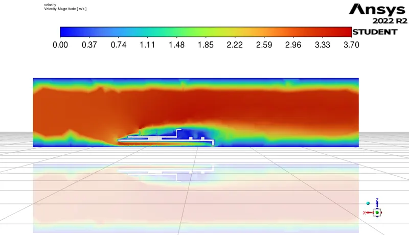
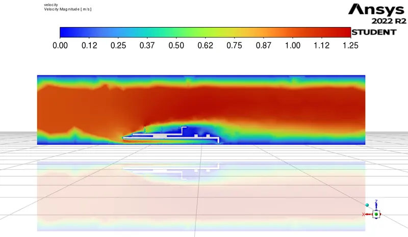
5.Velocity Contour

for Fine mesh

Fine mesh with U = 5m/s	Fine mesh with U = 3m/s	Fine mesh with U = 1m/s

for Coarse mesh

Coarse mesh with U = 5m/s	Coarse mesh with U = 3m/s	Coarse mesh with U = 1m/s

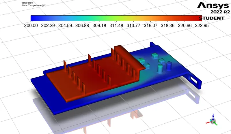
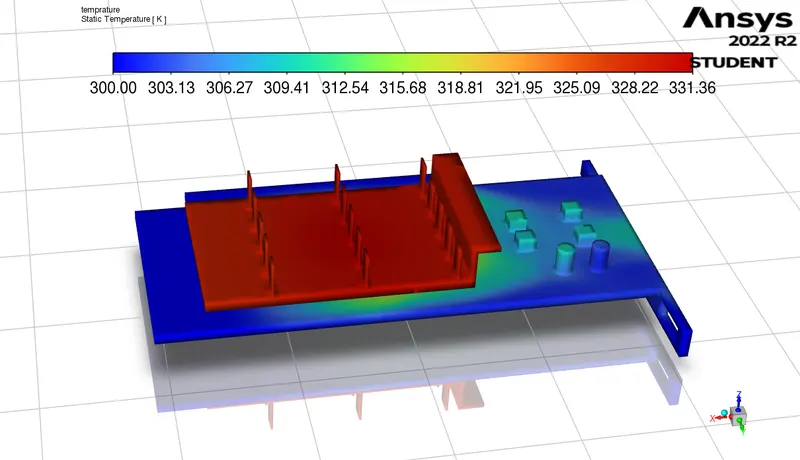
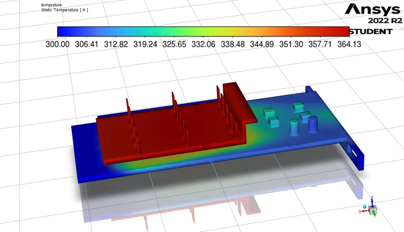
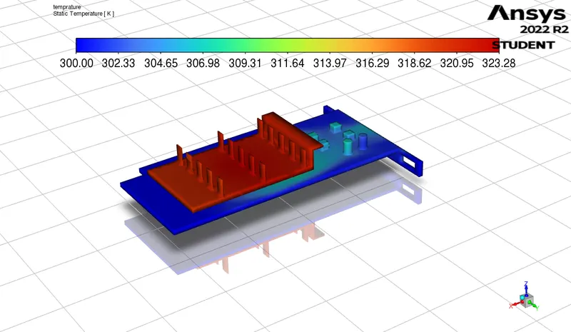
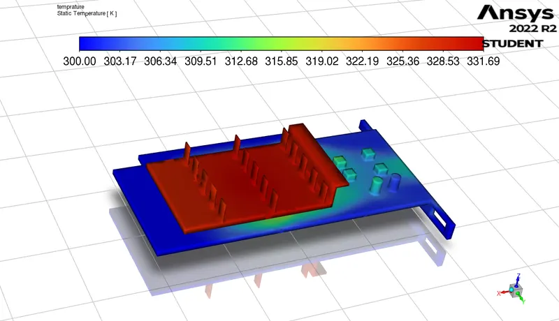
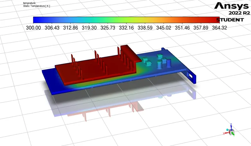
6.Hot zones

for Fine mesh

Fine mesh with U = 5m/s	Fine mesh with U = 3m/s	Fine mesh with U = 1m/s

for Coarse mesh

Coarse mesh with U = 5m/s	Coarse mesh with U = 3m/s	Coarse mesh with U = 1m/s

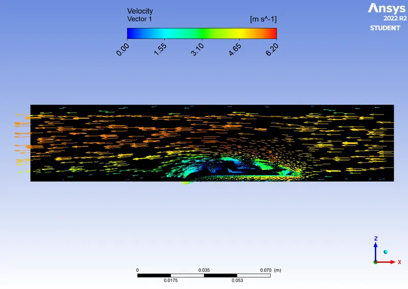
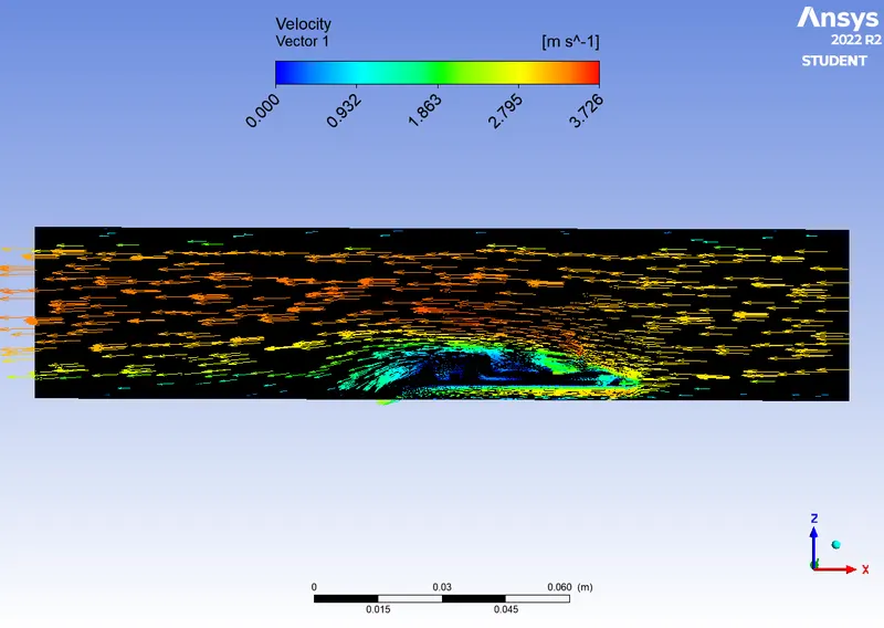
7.Velocity Vector

for Fine mesh

Fine mesh with U = 5m/s	Fine mesh with U = 3m/s	Fine mesh with U = 1m/s

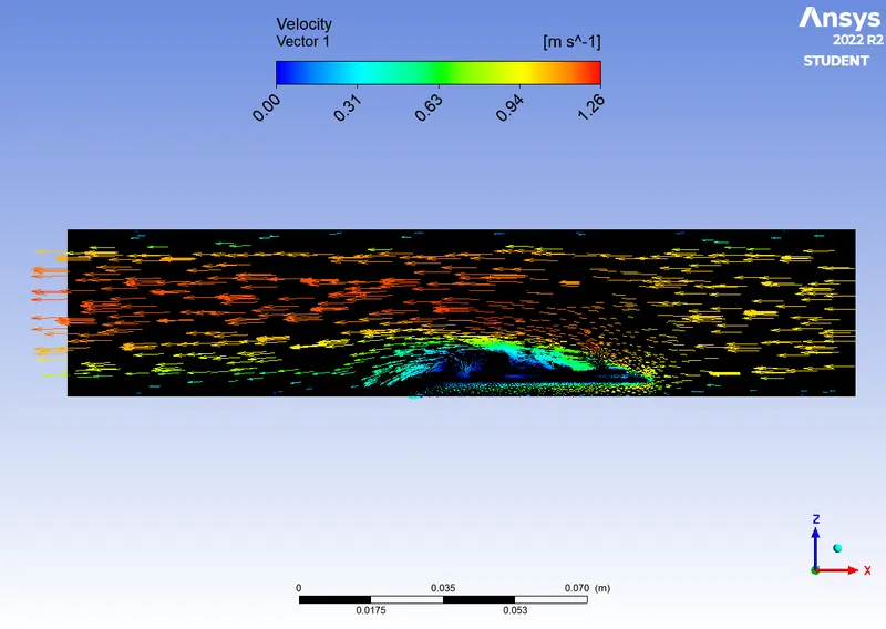for Coarse mesh

Coarse mesh with U = 5m/s	Coarse mesh with U = 3m/s	Coarse mesh with U = 1m/s

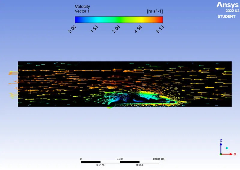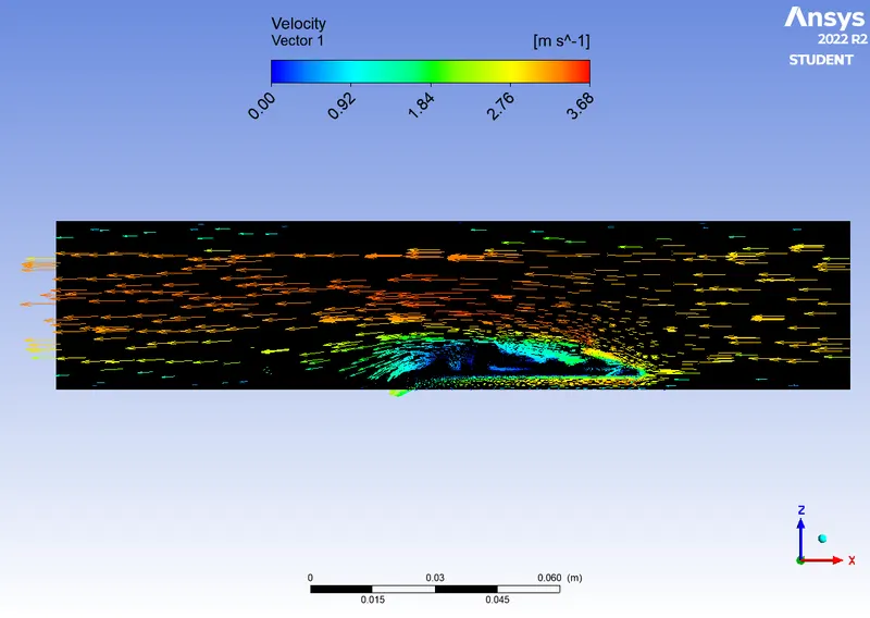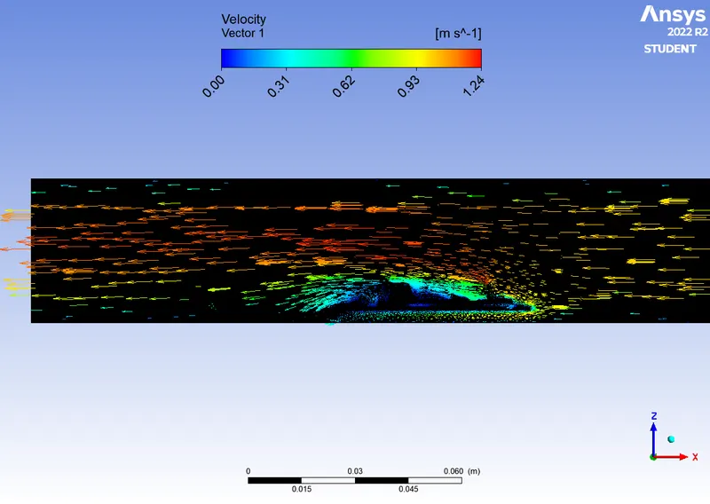8.Animation

for Fine mesh

Fine mesh with U = 5m/s	Fine mesh with U = 3m/s	Fine mesh with U = 1m/s

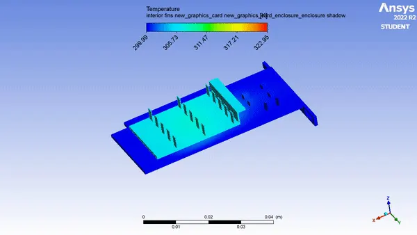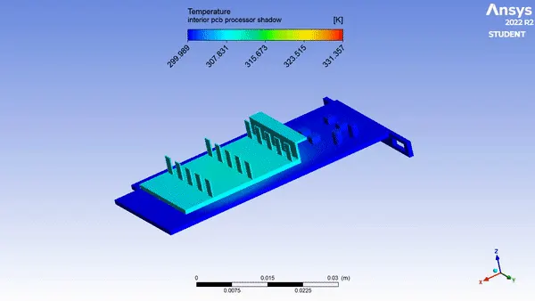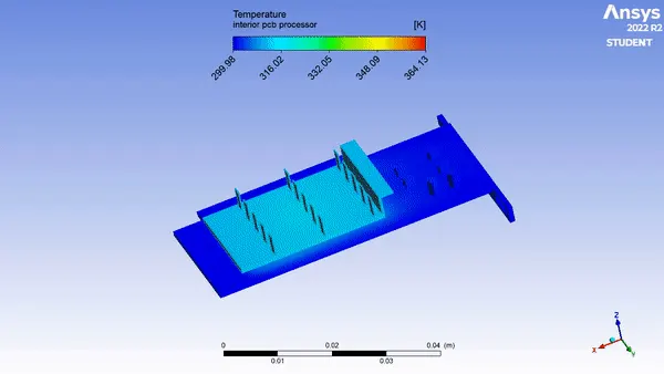for Coarse mesh

Coarse mesh with U = 5m/s	Coarse mesh with U = 3m/s	Coarse mesh with U = 1m/s

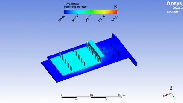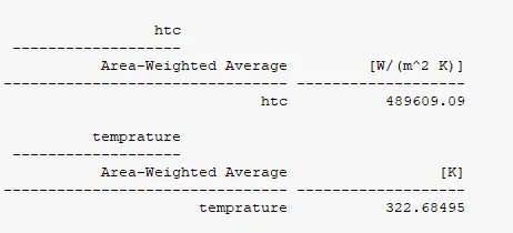
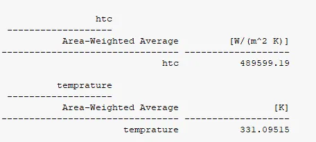
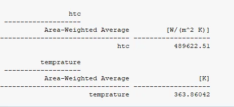
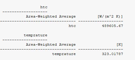
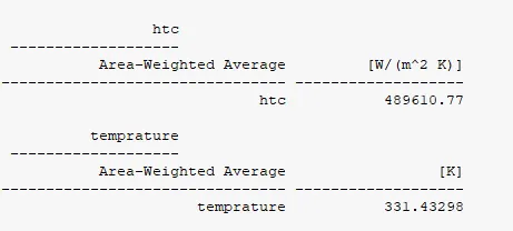
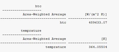
9.HTC and Temprature attend by the processsor

for Fine mesh

Fine mesh with U = 5m/s	Fine mesh with U = 3m/s	Fine mesh with U = 1m/s

for Coarse mesh

Coarse mesh with U = 5m/s	Coarse mesh with U = 3m/s	Coarse mesh with U = 1m/s

Inference

1. Temprature on the surface of pressor increases as the velocity of air decreases as we can see in when velocity is 5m/s average temprature at processer is about 322.68k and when we use velocity of air as 1m/s the temprature rise to 363.86k

2. The main hot points are preocessor and area which in direct contact with processor i.e. fin parts and pcb

3. When we are using coarse mesh we are not accurate results

4. Heat transfer coefficient maximum at velocity 1m/s

5. Main Heat producing source is processor

6. Velocity is zero when it comes in direct contact with the main component

7. Temprature is lower on right side as air coming from right to left direction