Week 6 - CHT Analysis on a Graphics card

Abstract:

The simulation of a graphics card is performed. Potential hotspot regions are found out. Maximum temperature reached is studied. A CHT study is performed.

Key words: Graphics card, Conjugate heat transfer , ANSYS fluent

Introduction:

Computational fluid dynamics and more specifically conjugate heat transfer (CHT) analysis can accurately predict heat transfer by simultaneous solving all the relevant solid and flow field heat transfer processes, for example: conduction through solids, free and forced convection in the gases/fluids and thermal radiation.

Flow chart :

• Geometry preparation
• Mesh generation
• Fluent set up
• Post-processing

Geometry:

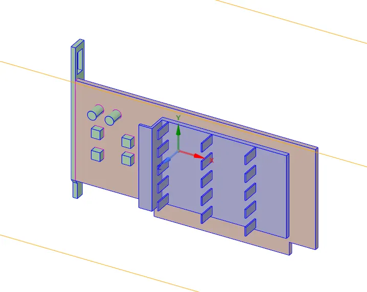
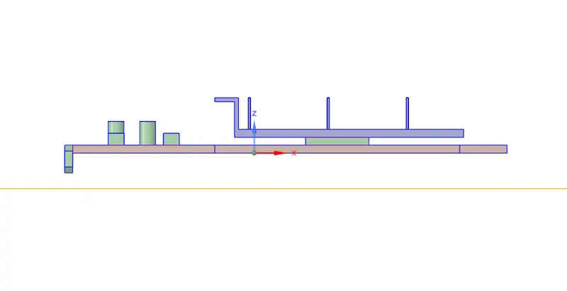
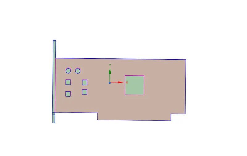
A step file is imported into ANSYS space claim. There are different components , namely:

1) Fin base

2) Fins

3) Processor

4) Enclosure

The processor:

Complete with enclosure:

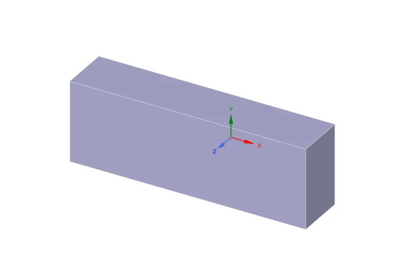
As there is a need of Conformal mesh, the share topology opyion is opted for. From the share option in Workbench. All the faces and edges that are common between the different components are shared

Meshing:

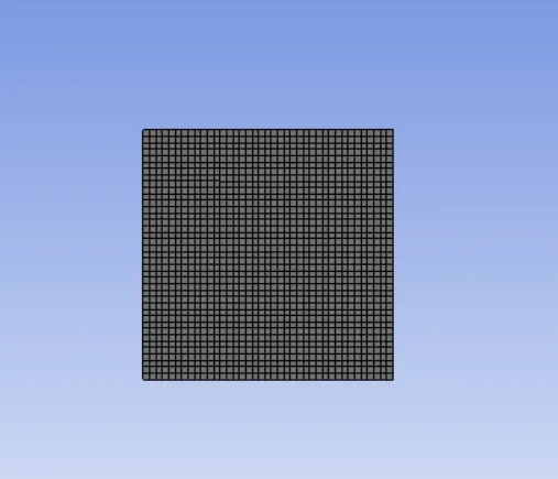
Processor is the main heat producing area. The fins and the processor are fine meshed using body sizing.

Processor:

Cut plane view:

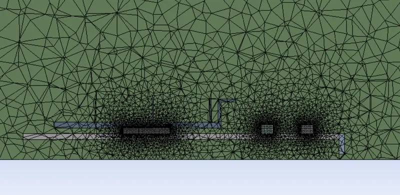
1.refined mesh:

nodes	664560
elements	457425
basic elemnt size	1e-002 meters
body sizing size	2e-004 meters

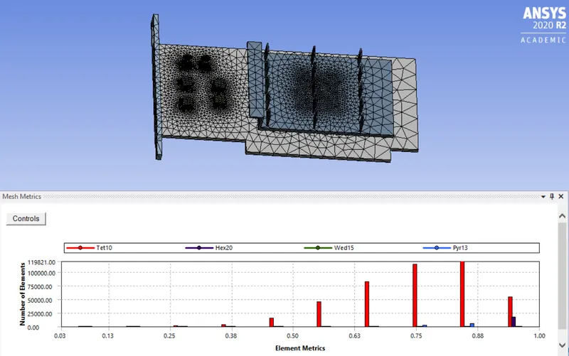
Orthogonal quality:

minimum	2.7725e-002
maximum	1
average	0.76423
standard deviation	0.13489

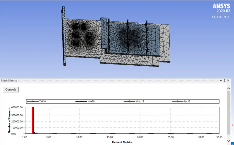
Aspect ratio:

minmimum	1.0243
maximum	32.994
average	1.861
standard deviation	0.5739

Element quality:

minimum	5.5794e-002
average	0.83182
standard deviation	0.10849
maximum	1

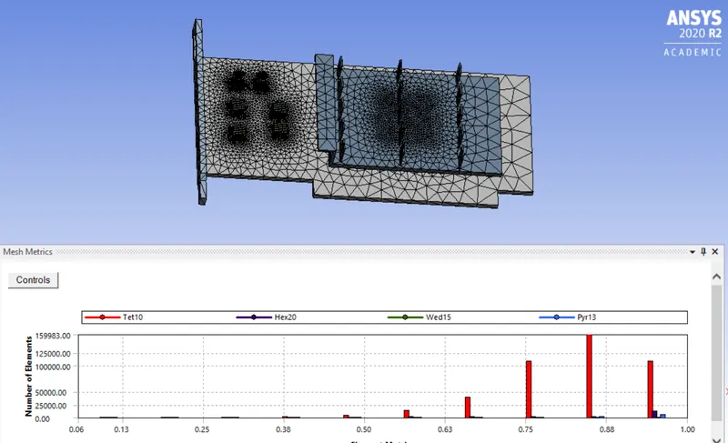
Skewness:

minimum	2.7725e-006
maximum	1
average	0.76423
standard deviation	0.13489

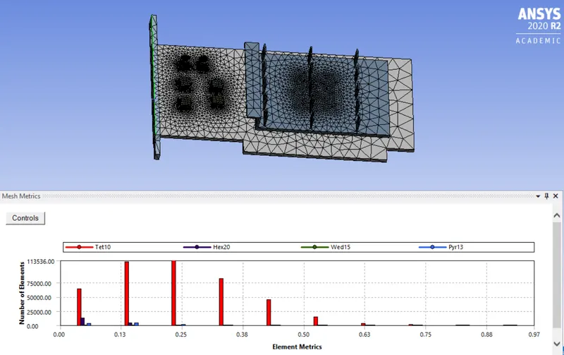
Heat transfer modelling:

The energy equation that is solved by ANSYS fluent is :

`(del)/(del(t))(rho*E)+nabla*(v*(rho*E+p))= nabla*(Keff*nabla*T-summationh(j)J(j)+(Teff*v))+S(h)`

In the above equation;

The first term of the LHS , `(del)/(del(t))(rho*E)` signifies the unsteady state .

The second term of LHS, `nabla*(v*(rho*E+p))`signifies the convection.

The first term of RHS , `Keff*nabla*T` signifies the conduction. K(eff) is the effective conductivity.

`Keff=K+Kt` where `Kt`is turbulent thermal conductivity.

`J(j)`is the diffusion flux of he species .

`T(eff)*v`signifies the viscous dissipation .

`S(h)`is the enthalpy source or sink.

In this project, steady state analysis is studied, so the `((del)/(del(t))(rho*E))`is 0.

Also, there are no species as conjugate heat transfer analysis is done, so `h(j)*J(j)`term is also equated to 0.

`E`is the energy per unit mass = `h-(p/rho)+(v^2/2)`

Pressure work and kinetic energy are always associated for with compressible flows, or when using density based solvers. While using pressure based solvers, they are omitted. They can be additionally put in by commands.

The Energy is turned on .

When fluid flows, it carries heat with it. This is called convection.

The rate of heat transfer is strongly dependent on fluid velocity. At the walls , heat transfer coefficient is calculated by the turbulent wall thermal functions.

`q(convection)=h*A(Tb-Tf)`

here `h`is the average heat transfer coefficient.

Conduction heat transfer is governed by Fouriers law .

`q = -k*nabla*T`

where `k`is the thermal conductivity.

For incompressible flows, viscous dissi[ation is neglected.

Thermal Wall boundary conditions:

There are six thermal conditions avalilable at the wall:

1) Heat flux

2) Temperature

3)Convection

4)Radiation

5) Mixed condition(Radiation +Convection)

6)System coupling(user defined)

Conjugate Heat Transfer:

At the fluid/solid or fluid/fluid interface a wall/wall-shadow is created by Fluent automatically while reading the mesh file. By default , energy is balanced on two sides of the wall.

It can be uncoupled and different thermal conditions on each side can be specified.

Fluent set up:

The meshed model is loaded into ANSYS Fluent. Required physics of the model is set:

Pressure based solver is used, as the flow is non compressible flow. Steady state analysis is done.

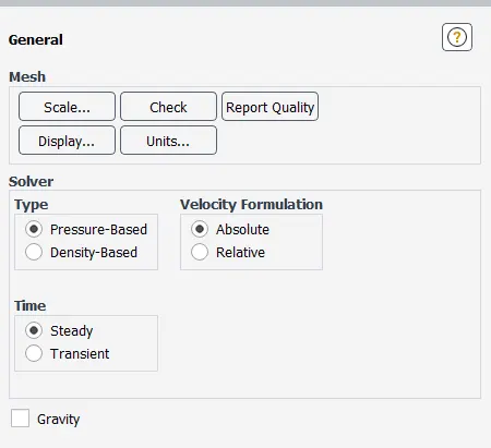
Energy is turned on.

Turbulence modelling:

A turbulent flow contains wide range of turbulent eddy sizes. These are accompanied by unpredictability. Energy is transferred from larger eddies to the smaller eddies.

The main aim is to find the time averaged velocity.

`u=u' + u(t)`

Here , u is the instantaneous velocity. u' is the fluctuating velocity and u(t) is the time averaged velocity.

Turbulence energy `k =((u'(t)^2+v'(t)^2+w'(t)^2))^0.5`

RANS approach basically solves the time averaged Navier stokes equations. All turbulent length scales are modelled here.

For two equaltion models, two transport equations are solved, giving two independent scales for calculating eddy viscosity.

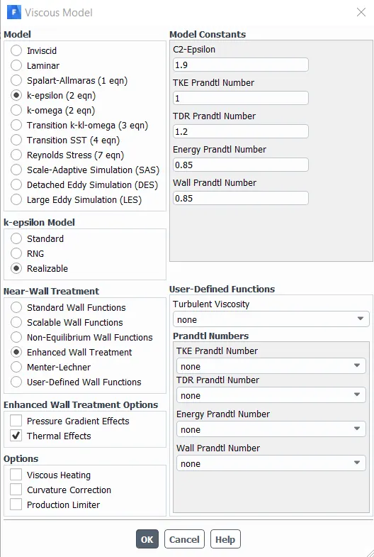
Realizable K epsilon model accurately predicts the spreading rate for both planar and round jets.

Velocity at inlet = 5m/s, 3m/s,1m/s

Material selection:

Base : Titanium

Fins and Fins base : Almuniium

Processor: Gold

	Density	Specific heat	Thermal conductivity
Gold	19320	129.81	297.73
Almunium	2719	871	202.4
Titanium	4850	544.25	7.44
Nickel	8400	460.6	91.74

Boundary Conditions:

Inlet:

Velocity normal to boundary is selected as 5 m/s,3m/s and 1m/s , Temperature as 300K

Others are kept at is

Cell Zones :

The enclosure is fluid , that is air.

Other cell zones are solid.

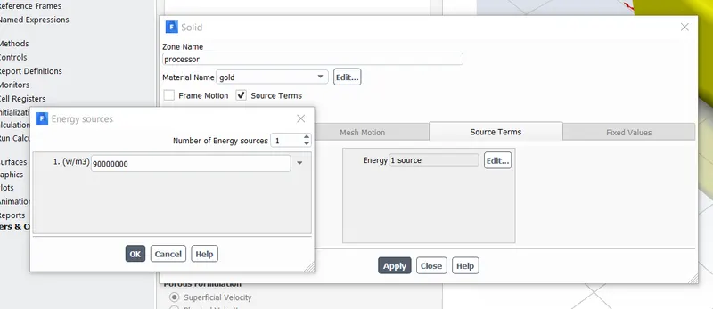
Processor . The processor acts as the source.

Here the Heat generated is 5.76 Watts. The volume of the processor is (0.008*0.008*0.001) m^3. So , the Source is given a constant value of ( 5.76/(0.008*0.008*0.001)) w/m^3 = 9e7

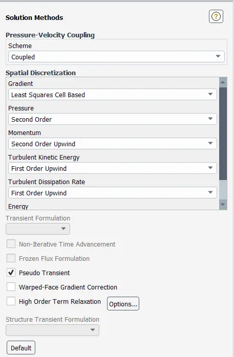
Solution methods:

Pressure velocity coupling : Coupled

Post processing:

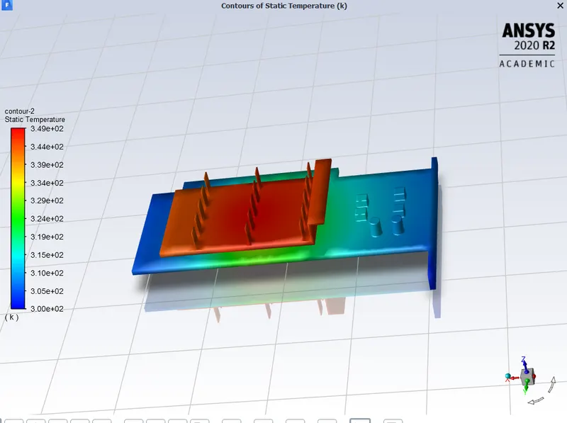
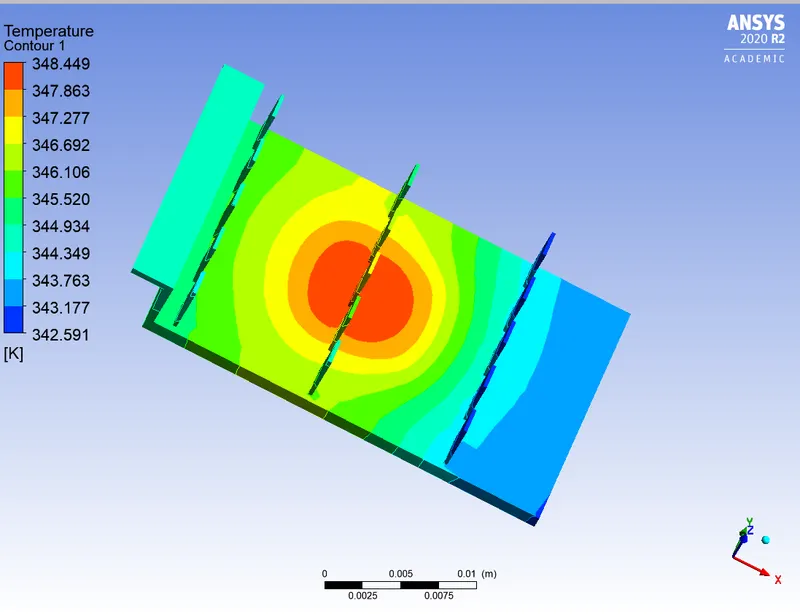
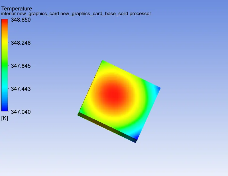
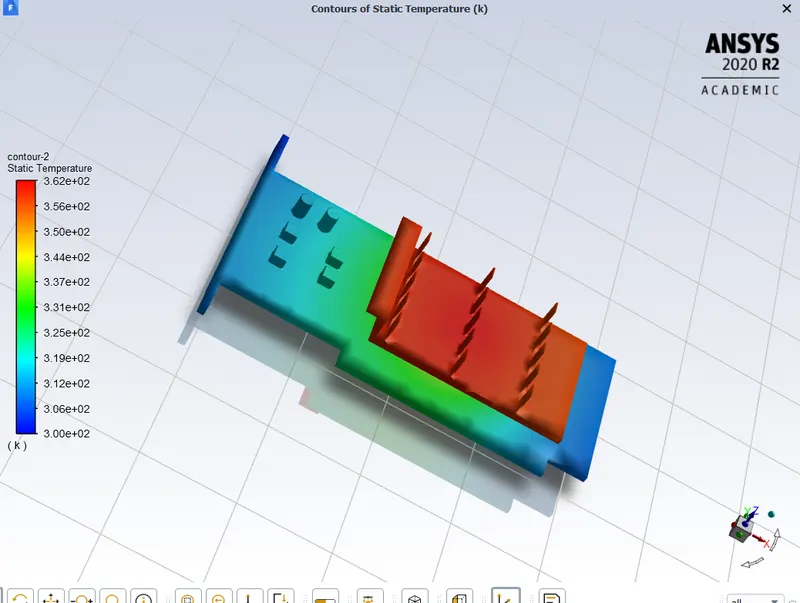
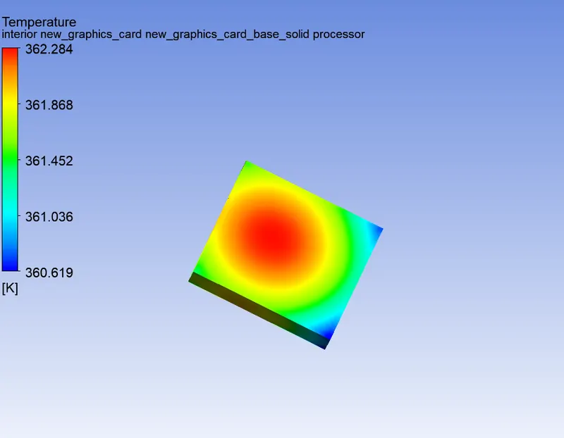
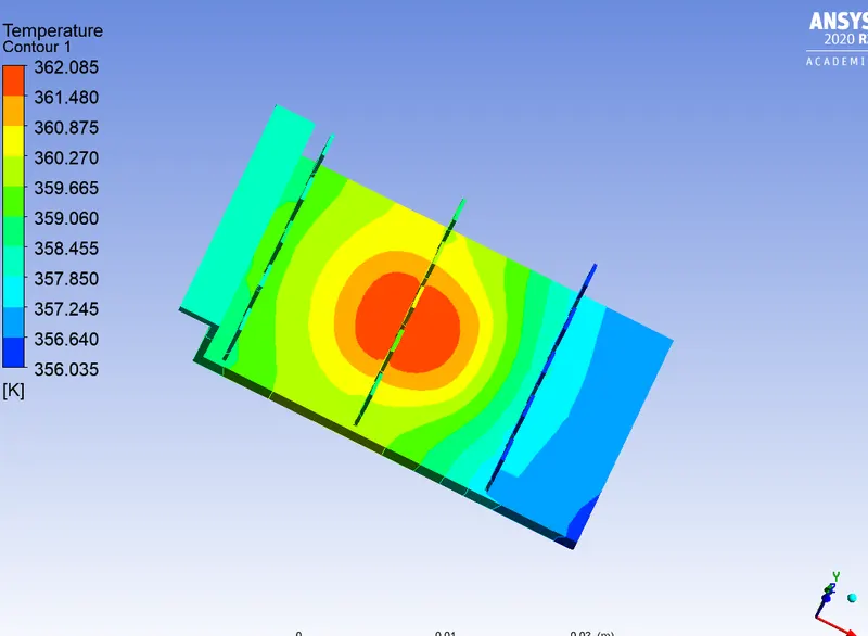
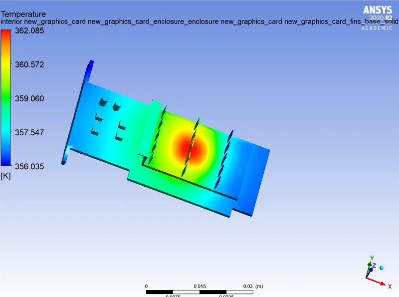
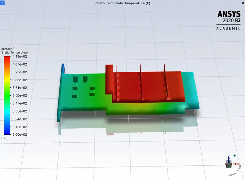
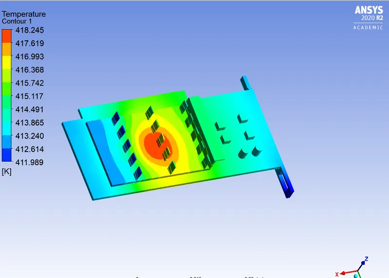
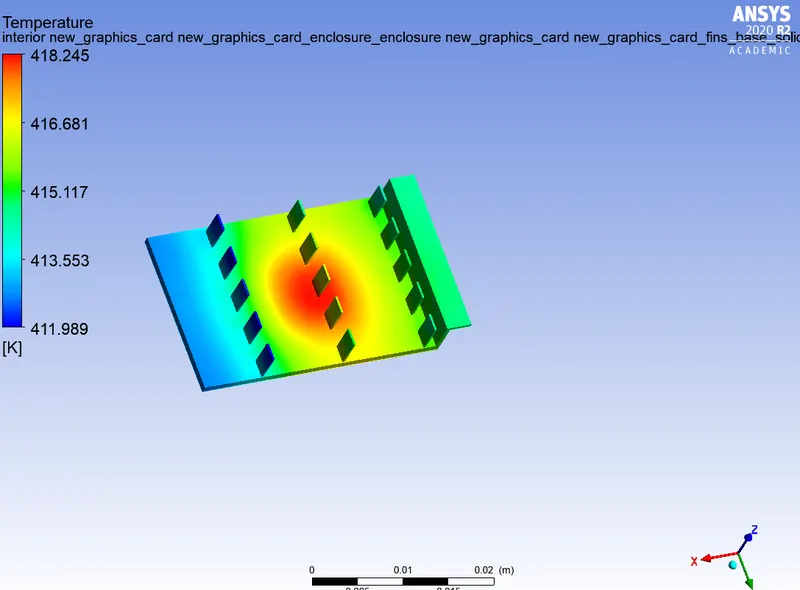
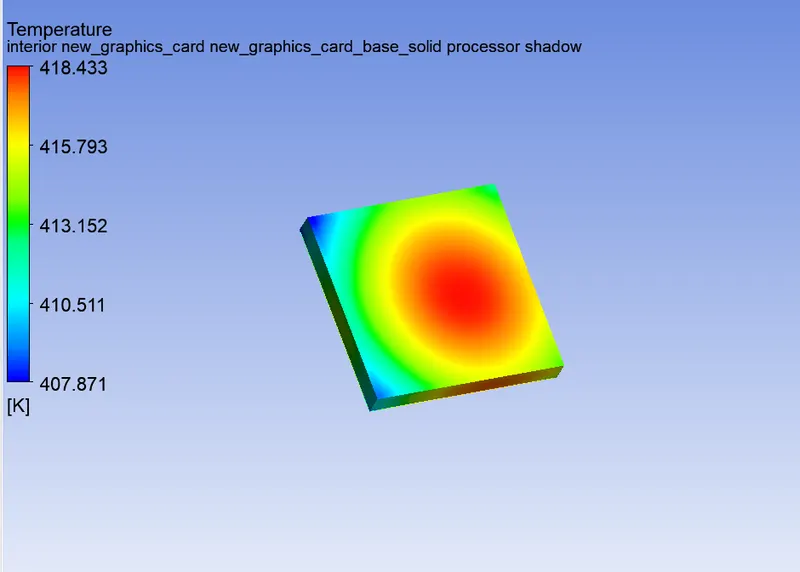
In CFD post, various contours are studied . The potential hotspots are foun out. Maximum temoerature reached also found out.

velocity 5m/s

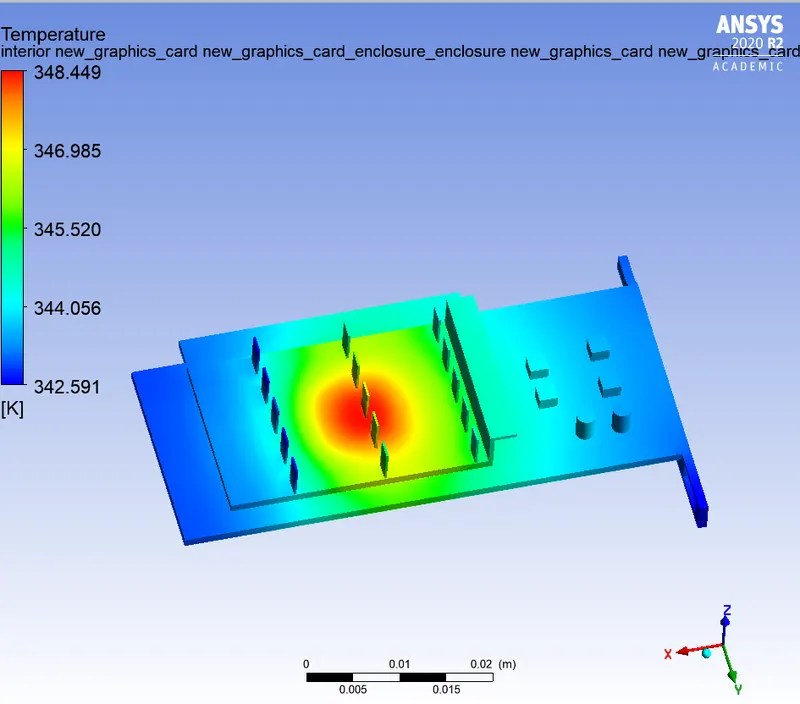
velocit = 3m/s

velocity 1m/s

Scaled residuals for velocity of flow 5m/s , 3m/s , 1m/s

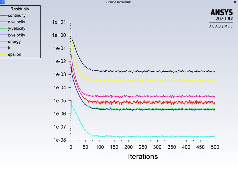
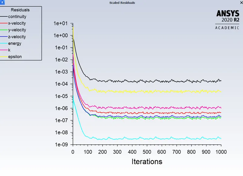
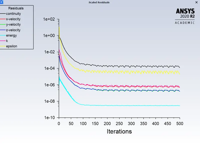
From the above plots , it can be inferred that the solution has converged.

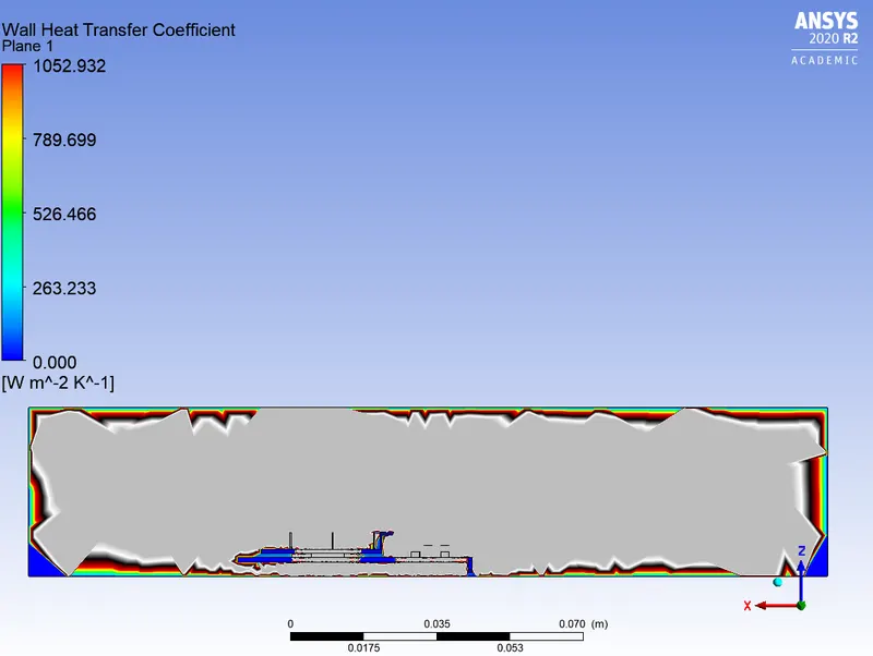
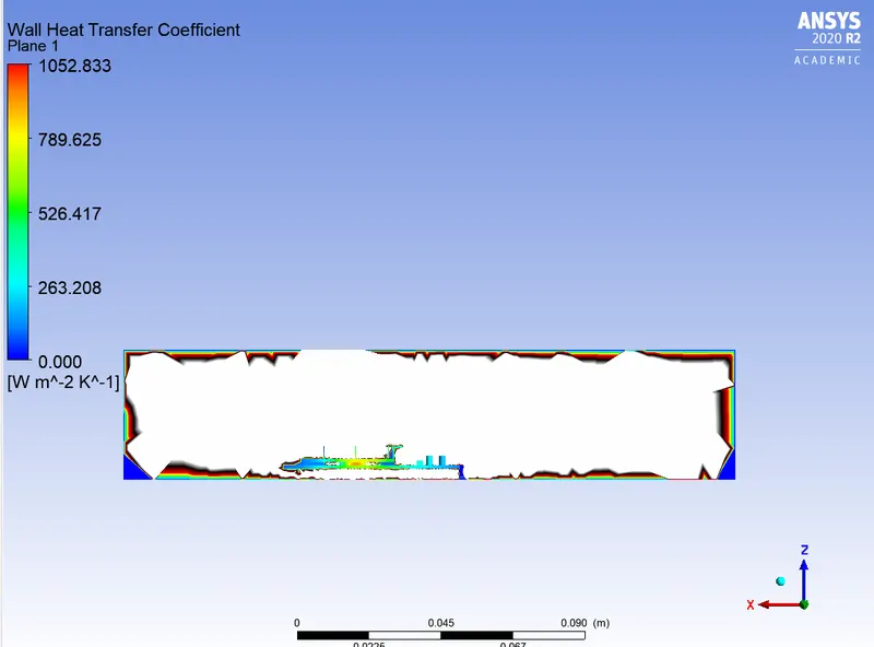
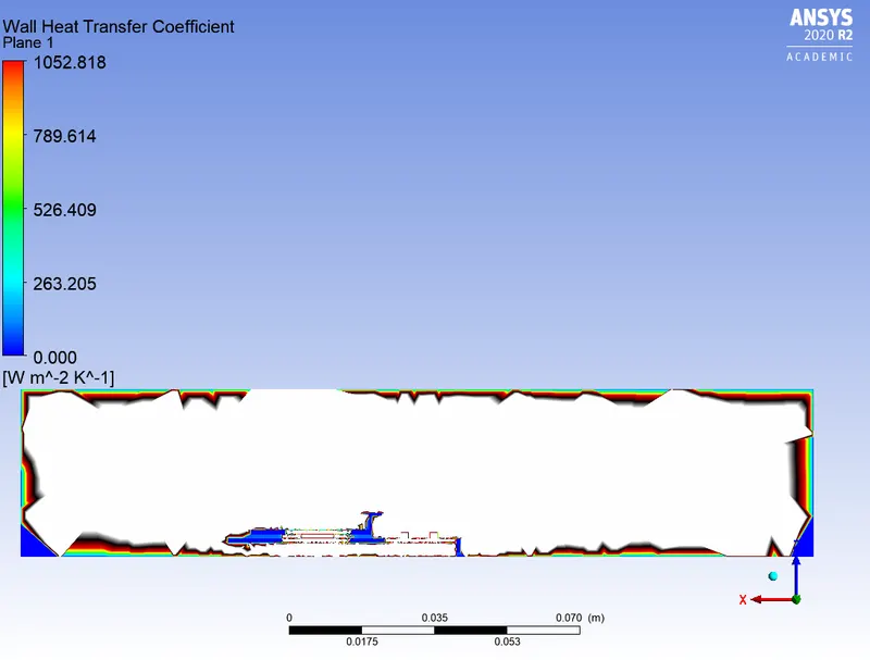
Wall heat transfer coefficient : for 5m/s ,3m/s,1m/s

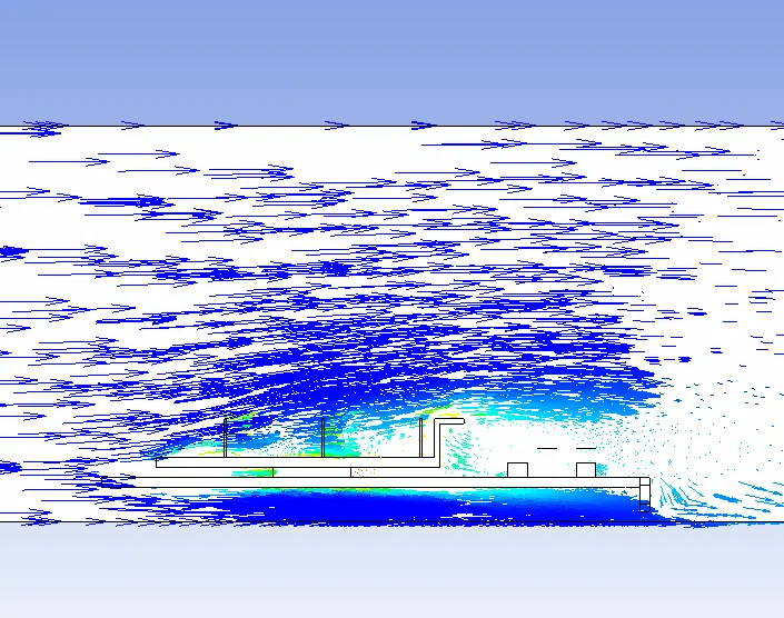
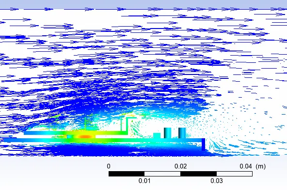
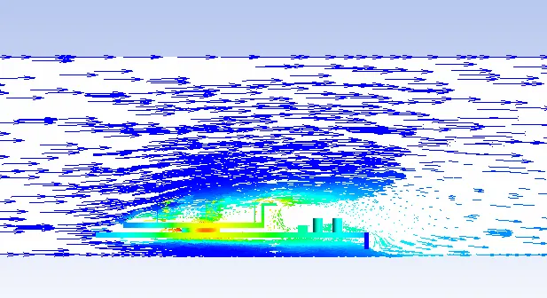
Vector plot of velocity in plane 1:

1) 5m/s 2)3m/s 3)1m/s

Results :

Velocity at inlet	5 m/s	3 m/s	1m/s
Maximum temperature	348.965 K	362.87 K	418.435 K
Maximum Wall Heat transfer coefficient	1052.93 W/m^2K^-1	1052.83 W/m^2K^-1	1052.82 W/m^2K^-1
Average Wall heat transfer Coefficient	129.77 W/m^2K^-1	128.563 W/m^2K^-1	127.538 W/m^2K^-1

Discussion:

• The potential hotspot for the graphics card is the processor region. Maximum temperature is reached in that region
• The Maximum temperature reached depends on the velocity of air at inlet. More the velocity, less is the maximum temperature reached.
• The wall heat transfer coefficient more or less remains constant with the variatiion of the velocity of air flow.