Week 6 - CHT Analysis on a Graphics card

Perform a steady-state conjugate heat transfer analysis on a model of a graphics card. You can use appropriate materials of your choice for the simulation. Make sure to properly define the correct solid and fluid zones.

Your Objectives:

1. Run the simulation by varying the velocity from 1m/sec to 5m/sec for at least 3 velocities and discuss the results.
2. Find out the maximum temperature and heat transfer coefficient attained by the processor.
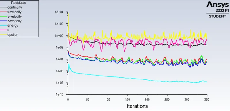
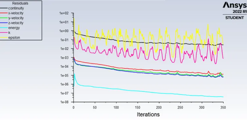
3. Prove that the simulation has achieved convergence with appropriate images and plots.
4. Identify potential hotspots on the model.

AIM : 

      To understand the concept of Conjugate Heat Transfer (CHT) Analysis.

Objective :

     To perform a CHT analysis in Graphics Card and to monitor the effect of velocity (Reynolds Number) on the heat transfer.

Heat Transfer Coefficient :

Empiricle Coorelation: 

• Reynolds Number :

Re=U∞⋅ρ⋅Lcμ">Re=U∞⋅ρ⋅LcμRe=U∞⋅ρ⋅Lcμ

• Prandtl Number:

Pr=Cp⋅μk">Pr=Cp⋅μkPr=Cp⋅μk

• Nusselt Number:

Nu=hLck">Nu=hLckNu=hLck

• Here k is thermal conductivity of fluid.
• Therefore, h (heat transfer coefficient) is a function of Re and Pr too.
• If the velocity U∞">U∞U∞ increases, the surface heat transfer coefficient is also going to increase.Therefore, the heat transfer is also going to increase.
• Idea in a nutshell, for our case, we must have higher heat transfer coefficient (h) in order to keep the processor cool.

Simulation Procedure:

Three cases were run for this setup.

• Case 1 : Velocity = 1m/s
• Case 2 : Velocity = 3 m/s
• Case 3 : Velocity = 5 m/s

CASE-1 : Velocity of 1 m/s

Geometry :

• Import the given geometry into the spaceclaim.
• Unable share topology in order to get conformal mesh.

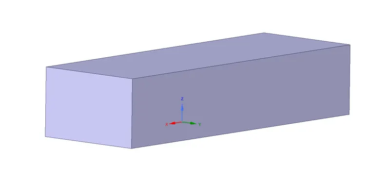
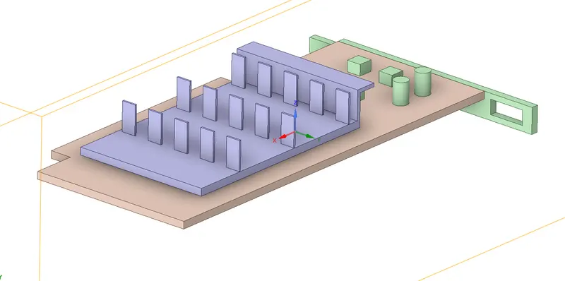
• Disable the encloser to see the graphic card.

Meshing:

• For this particular case mesh must be refined for the processor and the sink for better Temperature field values.
• Before, meshing, one must make sure the geometry assigned solid and fluid to appropriate bodies.
• Select geometry then new graphics card, select the component and assign as solid against 'fluid/solid'. Do this for all the components except the enclosure. Asign fluid for enclosure.
• Cut the plane by selecting the section plane tool.
• Then create named selection for the components as inlets, outlets, base, fins and processor. 

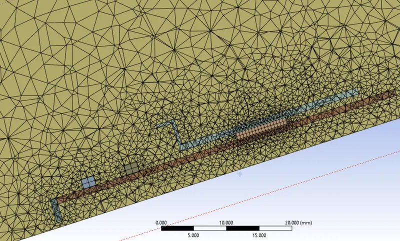
• Assign the top, bottom and the side walls as 'wall'.
• And the domain as 'flow_domain'.
• Now selec the porcessor and assign body sizing. Elemnt size = 0.4 mm
• Similarly do it for other parts of the graphics card.
• Then check the mesh statistics.

Setting up the physics :

• Make sure steady state is selected. over to 'Physics tab' and check the energy check box, conduct a 'k-epsilon model'.
• Select 'Material Edit/Create' tab.
• Select solid from dropdown menu. Select 'Fluent Database' then select aluminium and copy and give name as silicon.
• Similarly create a new material for base.

PROPERTIES OF MATERIAL CREATED:

• FR-4 : for base
• Silicon : for Processor
• Aluminium : for fins

• Go to cell zone and select processor. Check the 'source term' check box.
• For Energy assign one and a window will popup and give a value of 7,81,25,000 Wm3">Wm3Wm3. 5W divided by (8*10^-3*8*10^-3*10^-3) = 7,81,25,000.
• Select boundaries, select inlet and assign velocity value of 1 m/s.
• Go to 'soluitons' tab, select report definition and then select Surface Report  and Area Weighted Average then Wall fluxs then Surface Heat Transfer and then select the processor. Similarly instead of selecting Wall Fluxs, slect Temperature.
• Initialize the soluiton using Hybrid Initialization.
• Carry the simulation for 350 iterations. Finner the mesh faster will be the convergence.

RESULTS :-

CASE-1 :

Residual plot -1 :

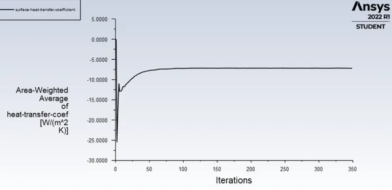
Surface heat transfer coefficient plot -1:

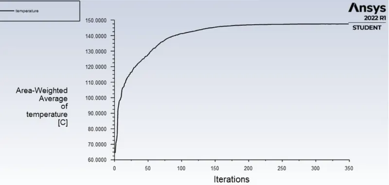
Temperature plot -1:

Contour plot -1:-

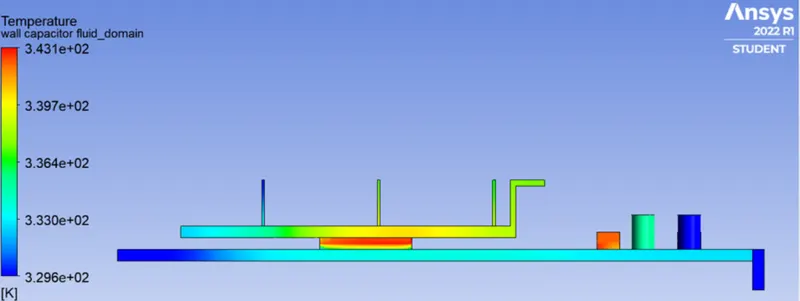
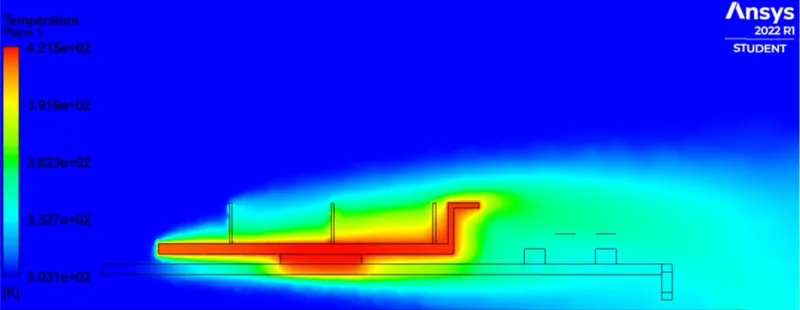
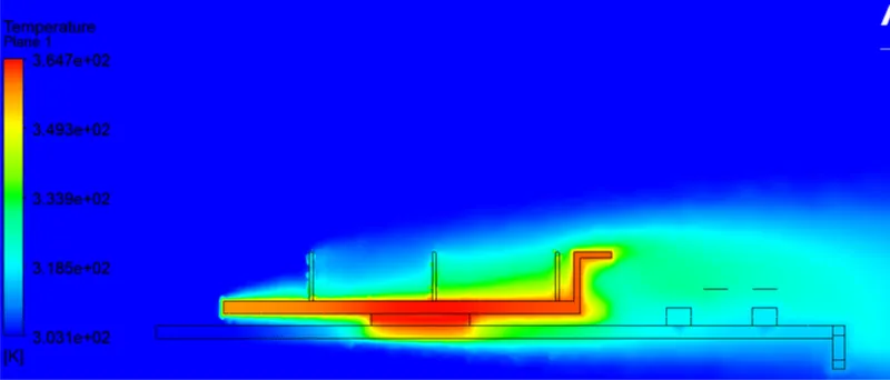
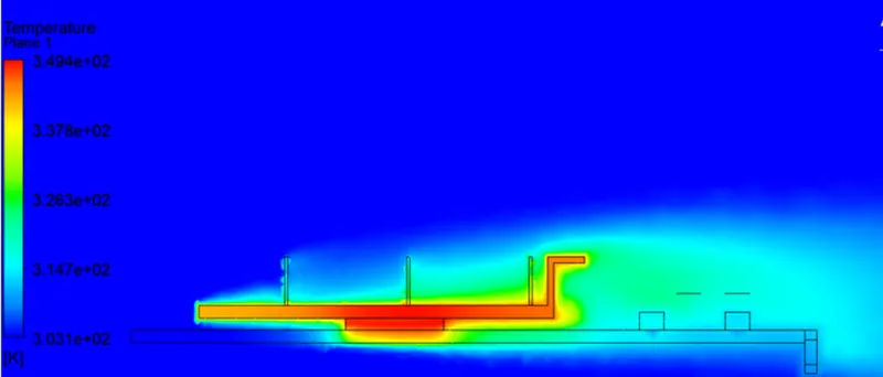
•  The hot spot is visible clearly above the processor and that is what is expected.
• The max temperature reached is 147.5161 C, which is very high for a processor.
• This must be taken care of by increasing the inlet velocity.

CASE-2 : Velocity 3m/s

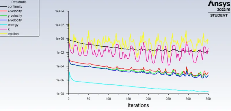
Residual plot-2 :

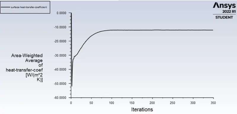
Surface heat transfer coefficient plot-2 :

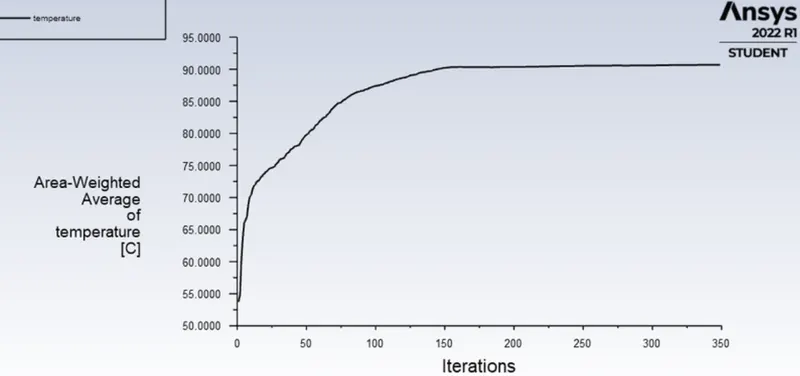
Temperature plot-2 :

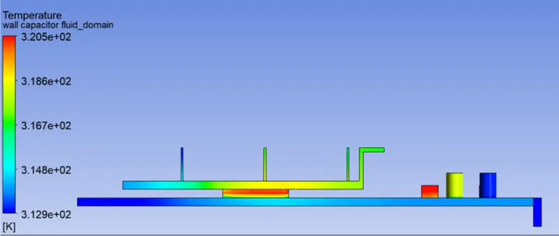
Contour plot-2 :

CASE-3 :Velocity 5m/s

Residual plot -3:

Surface heat transfer coefficient plot-3 :

Temperature plot -3:

Contour plots-3 :

Convergence : 

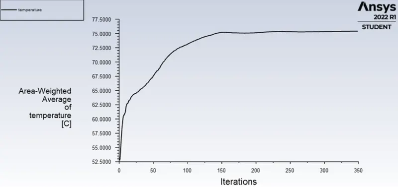
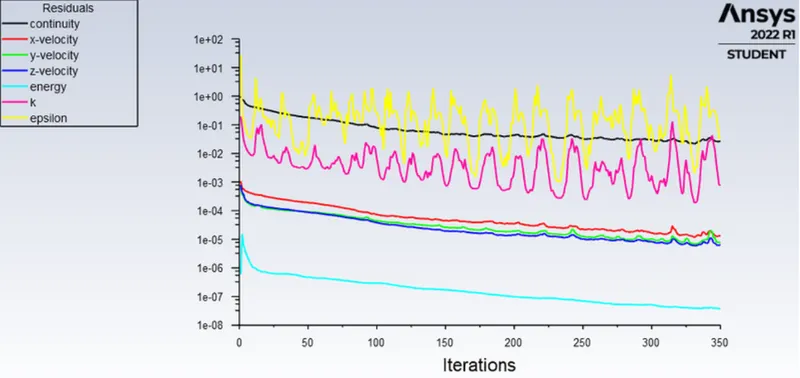
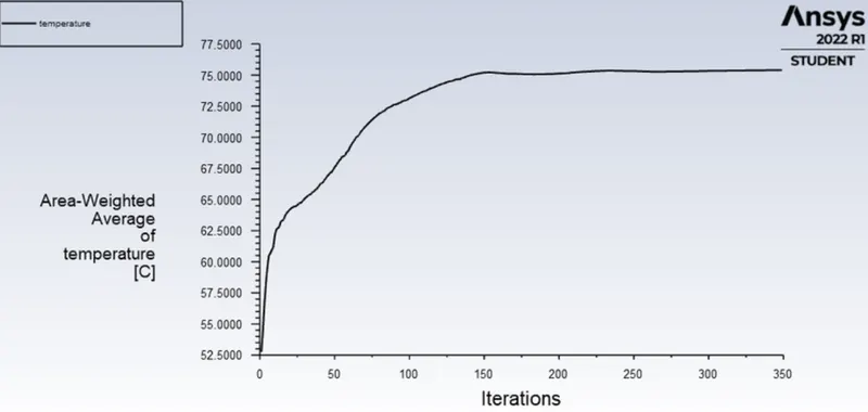
• Looking at the temperature plot, the temperature reaches steady-state after 150 iterations. This is the indication of solution being converged.
• But looking at the residual plot, the error is still big for a converged solution . This could be furthur refined by refining the mesh.

Potential Hotspots:

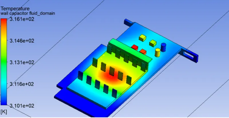
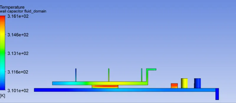
• All the three cases have hotspot near the processor and that is what we expect as it is the only component that is generating heat.

	case 1 (1 m/s)	case 2 (3 m/s)	case 3 (5 m/s)
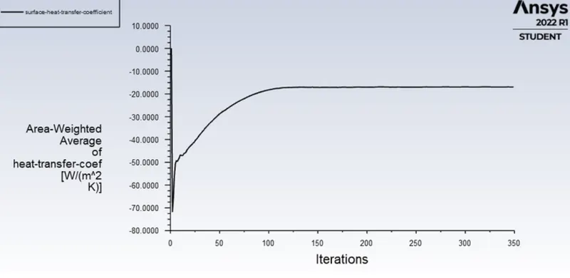
surface heat transfer coefficient	-7.1532	-12.2634	-16.9935
maximum temperature	146.98	90.6354	75.4360

• Therefore, Case 3 with velocity of 5 m/s maintains the temperature of the processor at 75 C.

Conclusion:

• The high temperatures are observed near the processor and the heat sink.
• Further,the mesh refinement is necessary for better results and simulations.
• It is quite evident that the temperature decreases with increase in veocity due to Reynolds-Nusselt-Prandtl Number relation.