Week 6 - CHT Analysis on a Graphics card

                                                      CHT analysis on the graphic card.

2. Objective –

• To Import graphic card CAD model in Spaceclaim and clean up the geometry
• To mesh it in Ansys Mechanical with suitable element size and quality.
• To apply proper boundary conditions, assign material and solve it with the proper model.
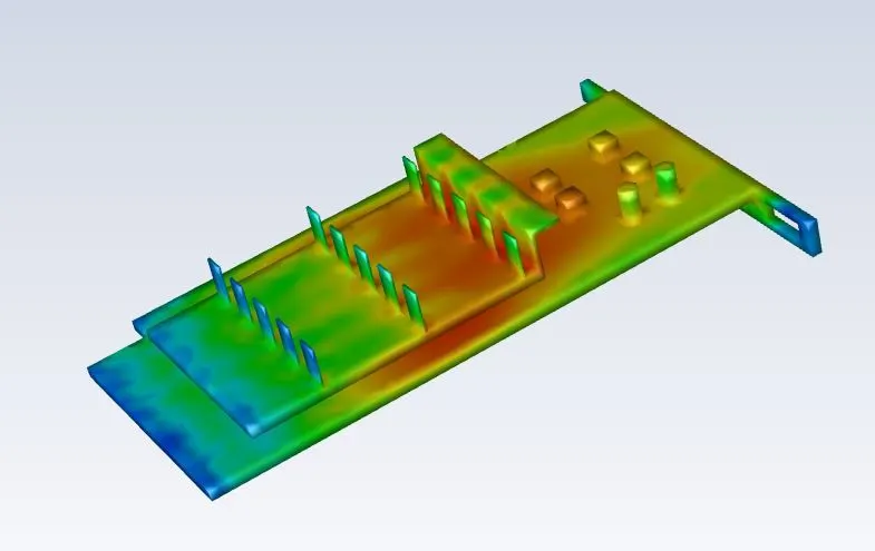
• To generate contours of temperature, heat transfer coefficient, and velocity and analyze it.

3. Theory –

Conjugate heat transfer is an analysis of heat transfer, the temperature where solids and fluids are exchanging heat. Through the analysis, engineers optimize the thermal characteristics for their chosen product design. Heat transfer in solids and heat transfer in fluids are combined in the majority of applications. This is because fluids flow around solids or between solid walls and because solids are usually immersed in a fluid. That way, CHT analysis has an important role in the CFD domain.

All electronic devices generate heat during their operation. Components and materials, used in these devices, have individual maximum temperature limitations. Therefore, thermal management is extremely crucial for system reliability and preventing failure. Simulation is a cost-efficient method to test different cooling strategies and optimize your solution. This is a great advantage to prevent time-consuming and expensive prototyping and physical testing procedure.

Someone can expect better results from mesh refinement but it does not work always because, After a certain value of element size, computation time will increase and it won’t affect the results much. A good mesh helps the computational fluid dynamics (CFD) solver converge to the correct answer while minimizing the computer resources expended. Every decent solver will yield an accurate answer with a good mesh, but it takes the most robust of solvers to get an answer on a bad mesh. So, in this study we will use different meshes for different components, processor and base will mesh with a fine mesh because we want a proper temperature distribution and feasible values of heat transfer coefficient. Encloser will have a little bit of coarser mesh than the processor because it will simulate the airflow. 

4. Procedure –

In this study, we simulated CHT on a graphic card and we generated the effect of air (Cooling fluid) velocity on the temperature of the processor. we assumed that the processor is consuming 145W(TDP) power in its peak performance and it has dimensions of 4cm*4cm*0.6cm. So, heat generated will be –

H = power consumption per unit volume

H = 145/(4*4*0.6*10^-6)

H = 1.52*10^7 W/m^3

Geometry –

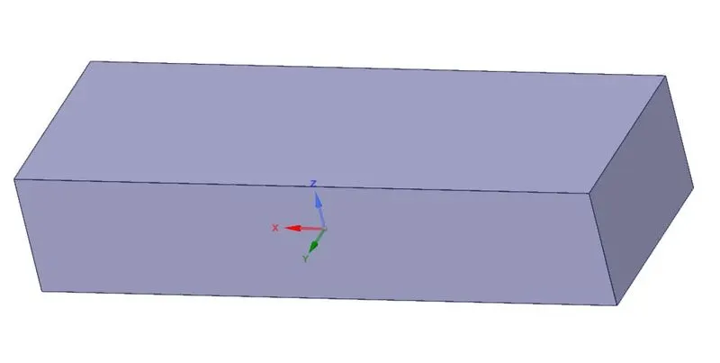
encloser- 

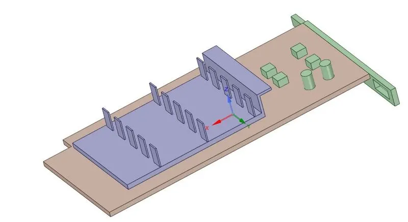
Processore and base -

Meshing –

Case1(Base) -

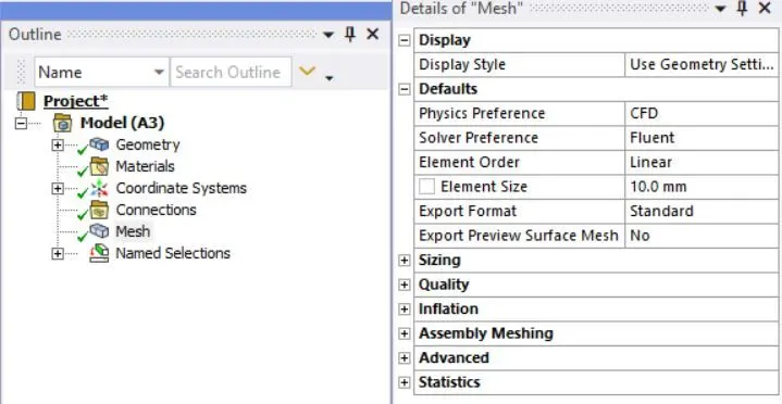
Mesh parameters -

Generated mesh -

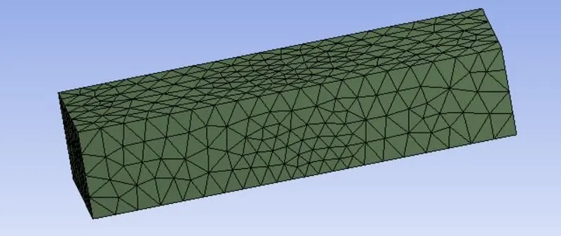
Encloser -

Processor and accesories -

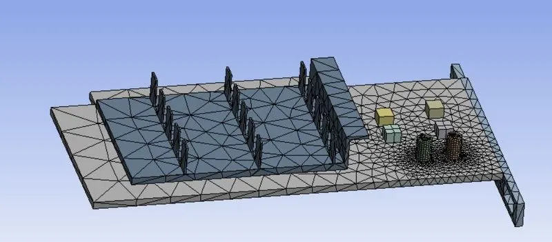
Closer view -

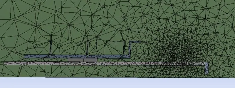
Case2 -

Mesh parameters -

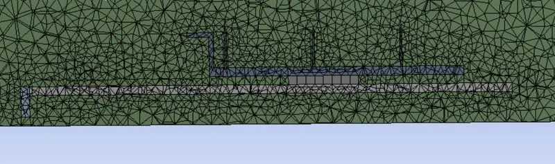
Body size 1 is used for enclose with element size 1mm and body sizing 2 is uesd for processor and accesories with element size of 1mm.

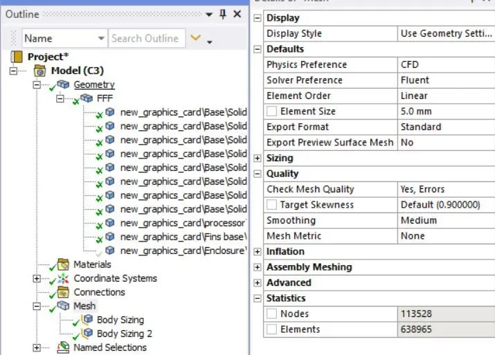
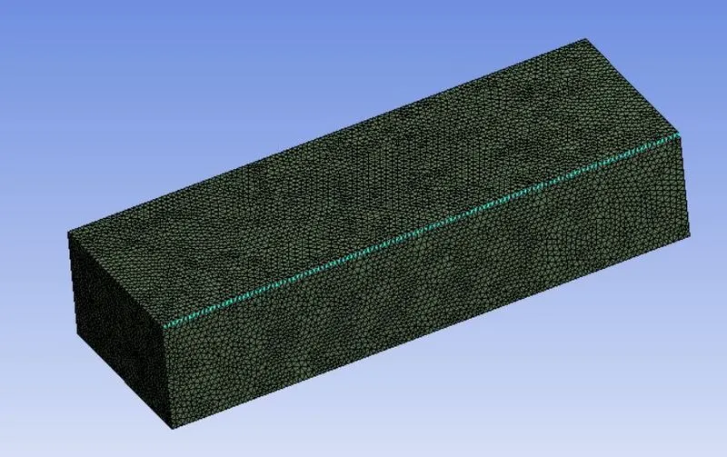
Generated mesh -

Encloser -

Processor and accesories -

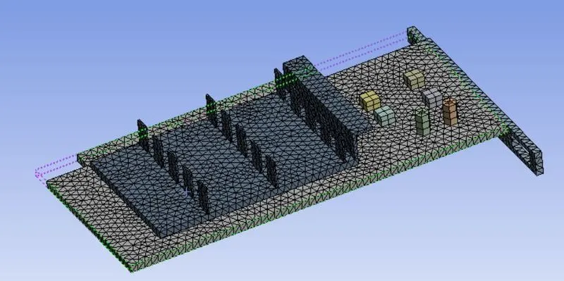
Closer look -

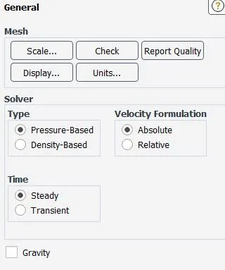
Solver setup –

Setting with be same each case air velocity.

General setting-

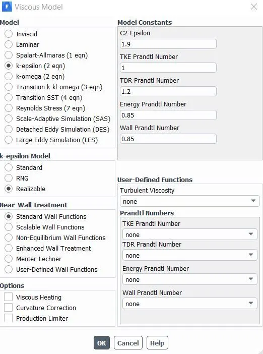
Solver model –

Materials setting –

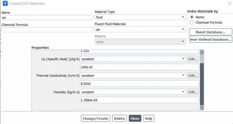
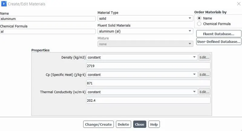
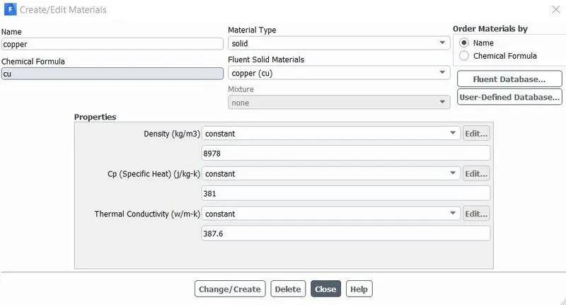
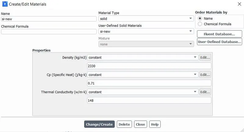
we assumed processor is made with silicon, base is made aluminium and fins are made with copper. air is used as cooling fluid.

Air properties -

Aluminium properties -

Copper properties -

Silicon properties -

Cell zone conditions –

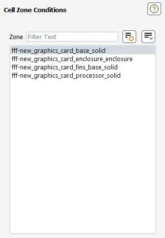
all the zones were treated as solid except encloser, which was treated as fluid. in processor's zone setting value of heat generation(H) and number of energy sources as one were given.

Boundary conditions -

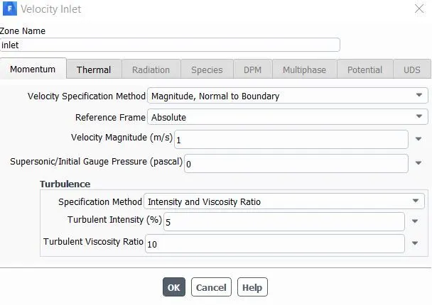
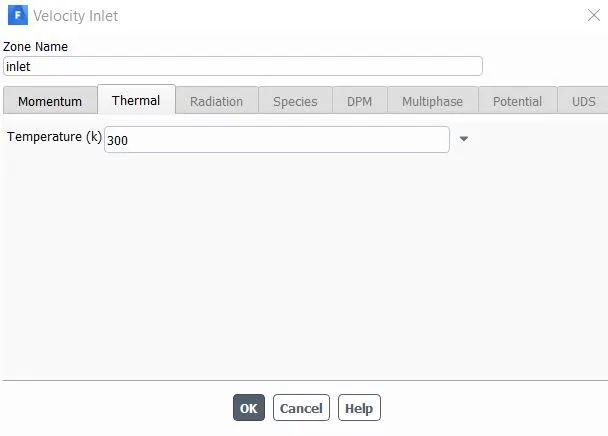
Simualtion conducted with three different velocities of air -1m/s,3m/s,5m/s

Results -

Case1(Base) -

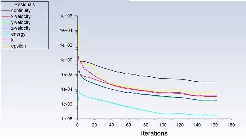
Residuals - 

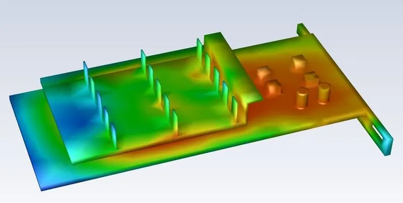
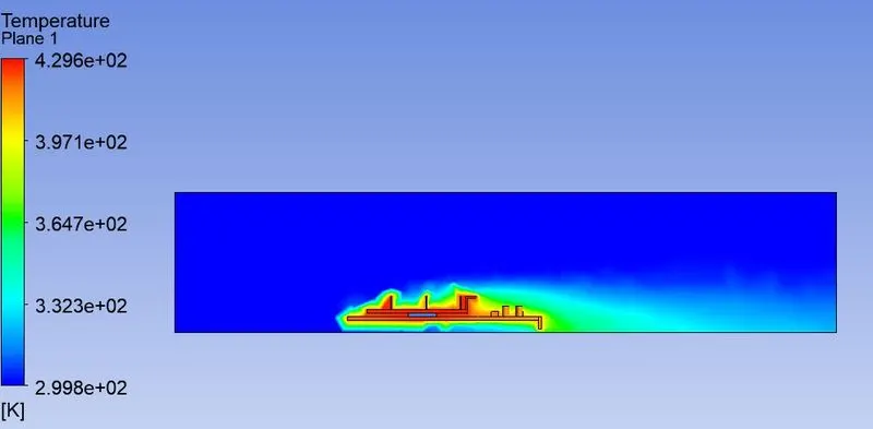
Temperature contour - 

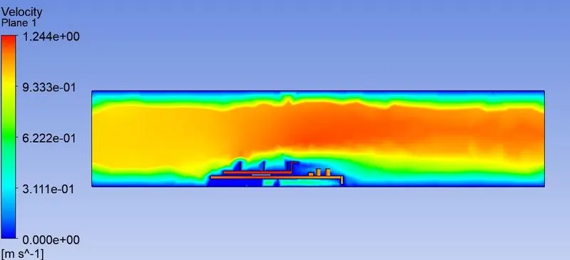
Velocity contour -

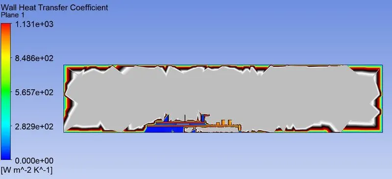
Heat transfer Coefficient - 

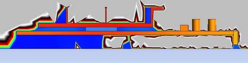
Case2 - (air velocity - 1m/s)

Residuals - 

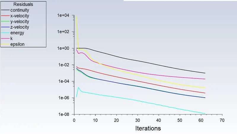
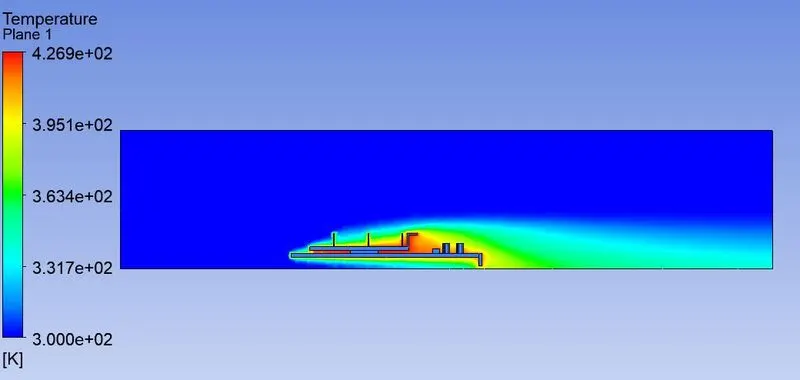
Temperature contour - 

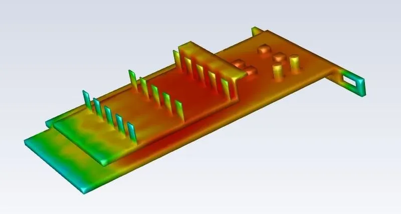
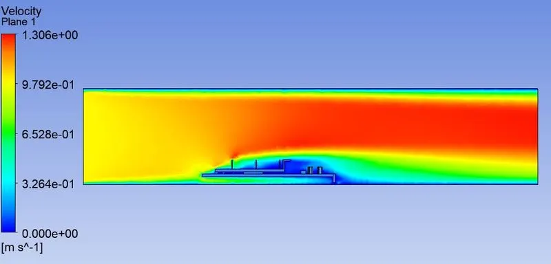
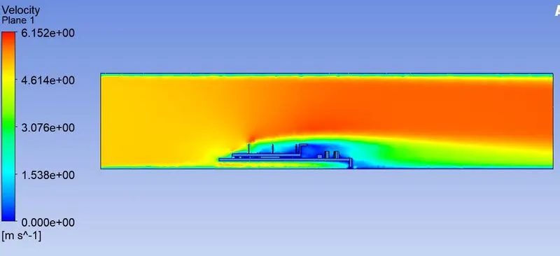
Velocity contour -

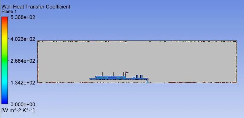
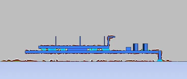
Heat transfer Coefficient - 

Case2- (air velocity - 3m/s)

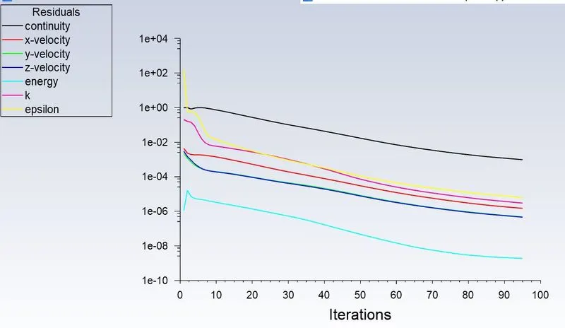
Residuals - 

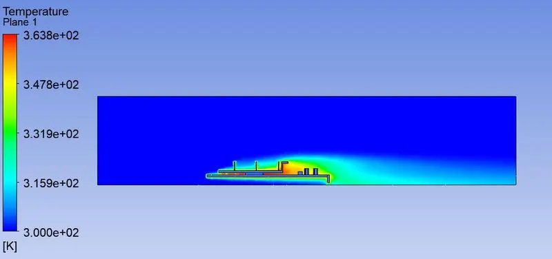
Temperature contour - 

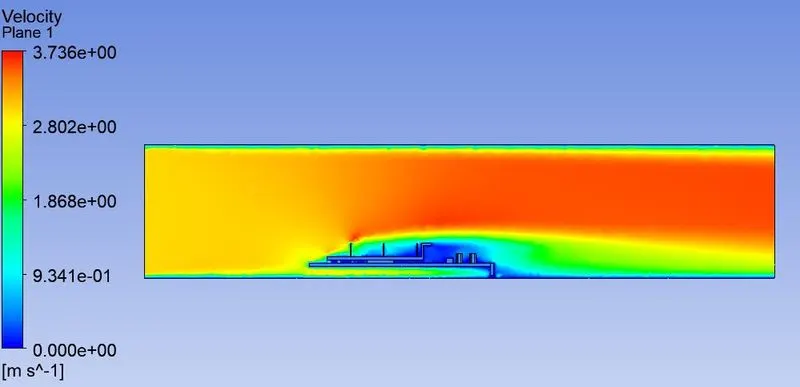
Velocity contour -

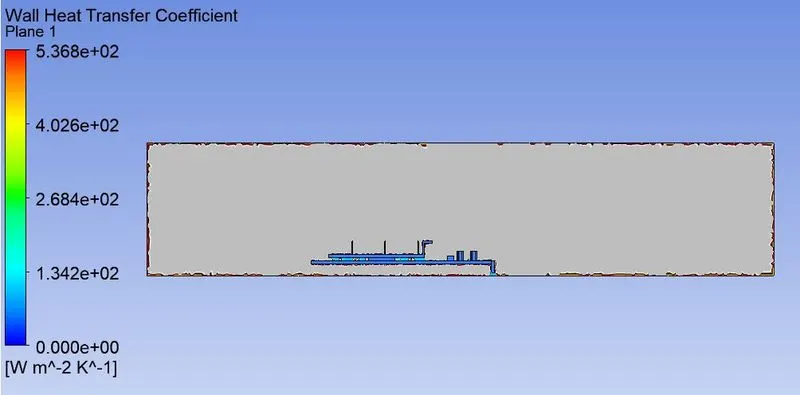
Heat transfer Coefficient - 

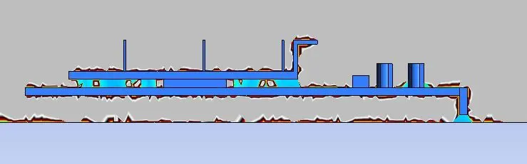
Case2- (air velocity - 5m/s)

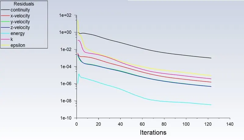
Residuals - 

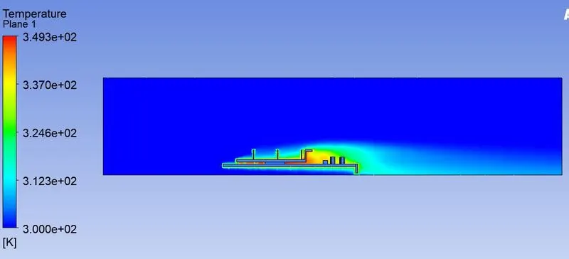
Temperature contour - 

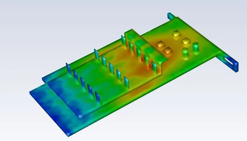
Velocity contour -

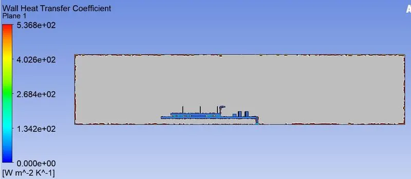
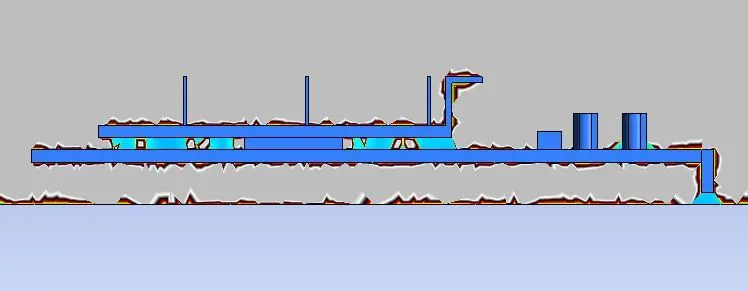
Heat transfer Coefficient - 

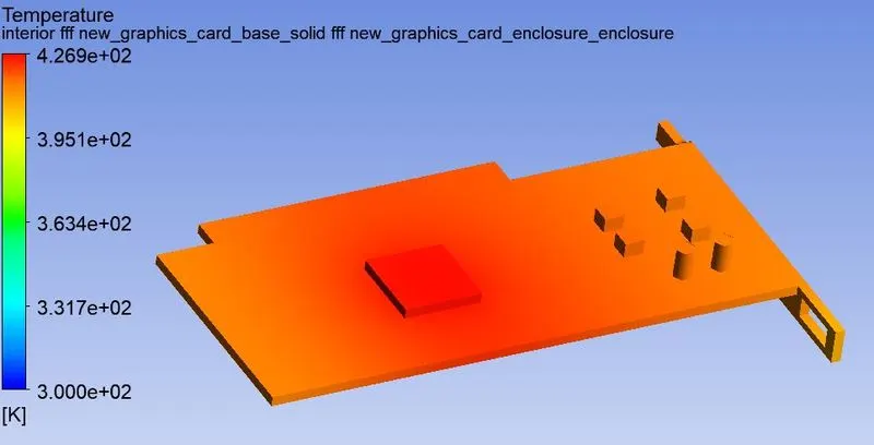
Hotspot represents hottest part of chip. In our simulation processor is sole component which is generating so it will possess maximum temperature, so it is a hotspot.

Result at a glance

Parameter/Case	Case1(Base)	Case2 with air velocity 1m/s	Case2 with air velocity 3m/s	Case2 with air velocity 5m/s
Number of the elements	84873	638965	638965	638965
Number of iterations for converge	163	62	95	123
Temperature (Max.) (K)	429.9	426.9	363.8	349.3
HTC (Max) W/m^2.K	1131	536.8	536.8	536.8

4. Conclusion –

The simulation was performed to find affect of cooling fluid velocity on temperature rise of processor and base.it can be seen from graph that maximum temperature is reduced by 66K by just increasing air velocity by 2m/s and temperature further reduces by 14K if we use air velocity as 5m/s. we know heat transfer is a boundary property and graph is indicting that heat transfer coefficient has got a significant reduction after refinement of mess. We can infer from it that heat transfer coefficient depends on the element size near boundary. The results are feasible and has proved some theories.