Week 3 - Solving second order ODEs

AIM:- to perform to solve second order ODE by using Matlab software

introduction;

A second-order ordinary differential equation is an ordinary differential equation in which any derivatives with respect to the independent variable have an order no greater than 2.

the ordinary differential equation helps us to solve many engineering systems. Such as harmonic motions, vibrations, damping, etc.

the second-order linear differential equation is used to model many systems in engineering.

let's consider

A simple pendulum consists of a mass "m"

hanging from a string of length "L"

from a fixed pivot point.

When displayed to an initial angle "`θ` and released.

the pendulum swings forward and backward with periodic motion.

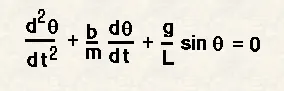
The equation is given by: is to solve the 2d odes equations

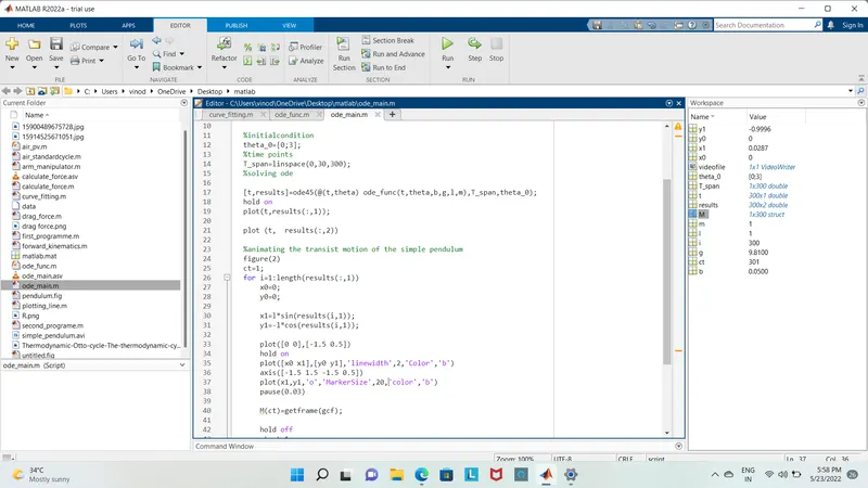
Explanation of the code

input are taken as given in problem

L=1 meter,

m=1kg,

b=0.05;

g=9.81 m/s^2

initial conditions taken as

Angular diaplacement =0,angular Velocity=3rad/sec,at time t=o

the motion is stimulated b/w 0-20 sec

solving ODE

ode solver ode45 is used in this Matlab program. The result is stored in an array of row matrix of two columns, for the value of displacement and velocity at different time periods,

ode-func is the function made to solve the given equation. where the assumptions are made in the form of code.

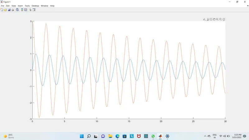
Figure(1)

plotting

the graph is plotted to get the waveform of the displacement and the velocity form from the initial conditions

FIGURE(2)

plotting

animating the transmit motion of the simple pendulum

to perform this operation we use for loop as the bob moves with a velocity and displaces for the different time of periods.And recorded it and animated the path of the oscillator

errors faced

we face the errors when we not using the hold on &hold off command in correct setup,

and at the pause code give the proper value

and give x0=0,y0=0,

and determine x1 andy1 values

main program

clear all

close all

clc

%inputs

b=0.05;

l=1;

g=9.81;

m=1;

%initialcondition

theta_0=[0;3];

%time points

T_span=linspace(0,30,300);

%solving ode

[t,results]=ode45(@(t,theta) ode_func(t,theta,b,g,l,m),T_span,theta_0);

hold on

plot(t,results(:,1));

plot (t, results(:,2))

%animating the transist motion of the simple pendulum

figure(2)

ct=1;

for i=1:length(results(:,1))

x0=0;

y0=0;

x1=l*sin(results(i,1));

y1=-l*cos(results(i,1));

plot([0 0],[-1.5 0.5])

hold on

plot([x0 x1],[y0 y1],'linewidth',2,'Color','b')

axis([-1.5 1.5 -1.5 0.5])

plot(x1,y1,'o','MarkerSize',20,'color','b')

pause(0.03)

M(ct)=getframe(gcf);

hold off

ct=ct+1;

end

%making the video file

movie(M)

videofile=VideoWriter('simple_pendulum.avi');

open(videofile)

writeVideo(videofile,M)

close(videofile)

function program for solving the ODE

function [dtheta_dt]=ode_func(t,theta,b,g,l,m)

theta1=theta(1);

theta2=theta(2);

dtheta1_dt=theta2;

dtheta2_dt=-(b/m)*theta2- (g/l)*sin(theta1);

dtheta_dt=[dtheta1_dt;dtheta2_dt];

end

OUTPUT

the animated simple pendulum

https://drive.google.com/file/d/1-69JUX-n5I3qaIvNSFNBxrcXgAG8NzPV/view?usp=sharing

CONCLUSION

by performing the above codes in Matlab we get the graph values and animated movie video