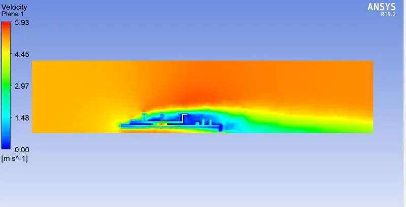
Week 6 - CHT Analysis on a Graphics card
Aim:
Perform a steady-state conjugate heat transfer analysis on a model of a graphics card.
Description:
The Conjugate Heat Transfer (CHT) analysis type allows for the simulation of heat transfer between solid and fluid domains by exchanging thermal energy at the interfaces between them. Typical applications of this analysis type exist as, but are not limited to, the simulation of heat exchangers, cooling of electronic equipment, and general-purpose cooling and heating systems.
Examples:
HVAC, Heat Exchanger, Tank, Internal Combustion Engine, Heat Sink, Boiler, Reactor, Heat Pipe, Turbocharger.
- Heat Transfer in a Solid - Conduction: Diffusion of heat due to temperature gradients in solids. A measure of the amount of conduction for a given gradient is heat conductivity. Conduction is described by Fourier’s law defining the conductive heat flux, q, proportional to the temperature gradient
- Heat Transfer in a Fluid - Convection: When heat is carried away by moving fluid. The flow can either be caused by external influences, forced convection or by buoyancy forces, natural convection.
Due to the fluid motion, there are three contributions to the heat transfer:
1. Convective contribution: Depending on the properties of the fluid and its region of flow, the domination of conduction and convection varies.
2. Viscous effects: Due to the fluid flow, the viscosity creates heat. This effect is often neglected due to its negligible value but should be taken into account for high-velocity cases.
3. Density effects: When the density becomes related to the temperature, the domain will have different densities at different locations based on the temperature distribution. This variation in density can cause the compression which in-turn generates the heat.
The contemporary conjugate convective heat transfer model was developed after computers came into wide use in order to substitute the empirical relation of proportionality of heat flux to temperature difference with heat transfer coefficient which was the only tool in theoretical heat convection since the times of Newton. This model, based on a strictly mathematically stated problem, describes the heat transfer between a body and a fluid flowing over or inside it as a result of the interaction of two objects. The physical processes and solutions of the governing equations are considered separately for each object in two subdomains. Matching conditions for these solutions at the interface provide the distributions of temperature and heat flux along the body–flow interface, eliminating the need for a heat transfer coefficient. Moreover, it may be calculated using these data.
Simulation Procedure:
Open Ansys workbench and drag the Fluid Flow(Fluent) to main window.
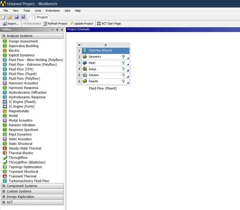
Go to geometry to import the geometry file.
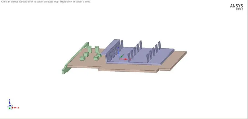
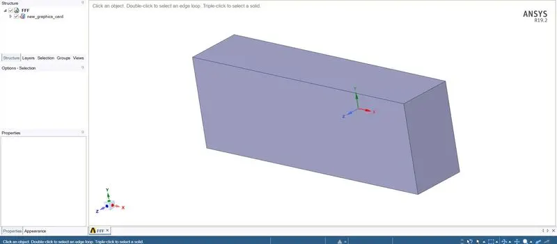
Then go to workbench option Click share perp tp change the Share topology.
Then update geometry in main window. After that go to mesh.
Select the faces by using selecting face option then name the faces like “Inlet, Outlet,Symmetry wall”, same as select the slid bodies and name them as " processor, fins, base".
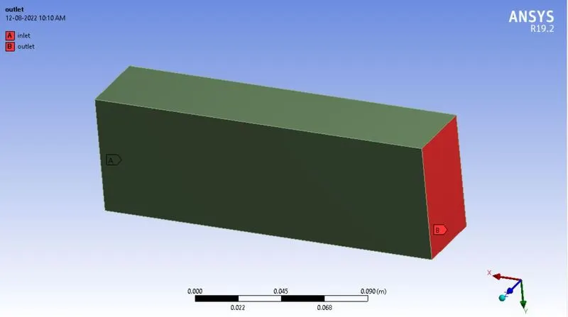
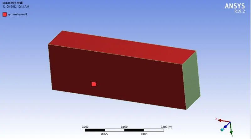
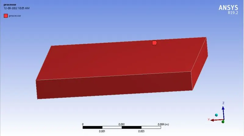
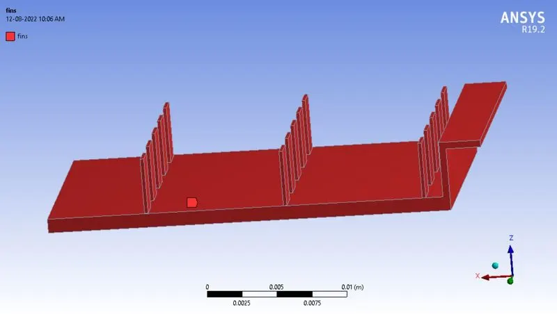
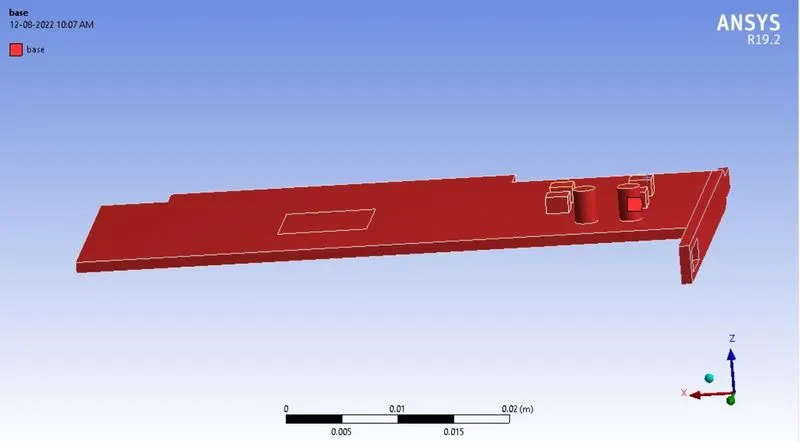
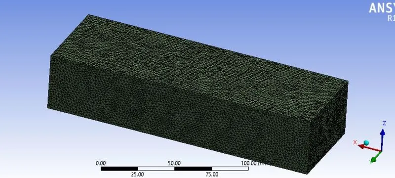
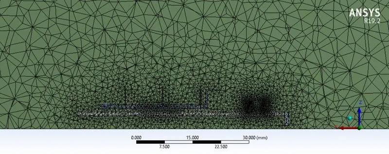
Then create a appropriate mesh by insert the body mesh and change the mesh size based on the component. Then generate the mesh.
Baseline mesh:
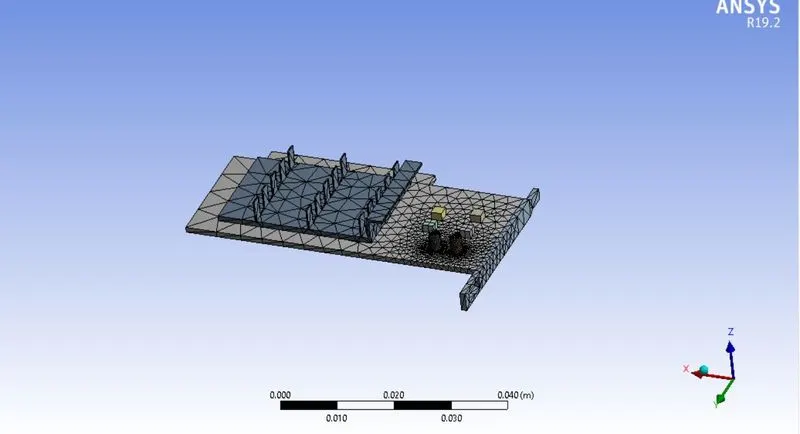
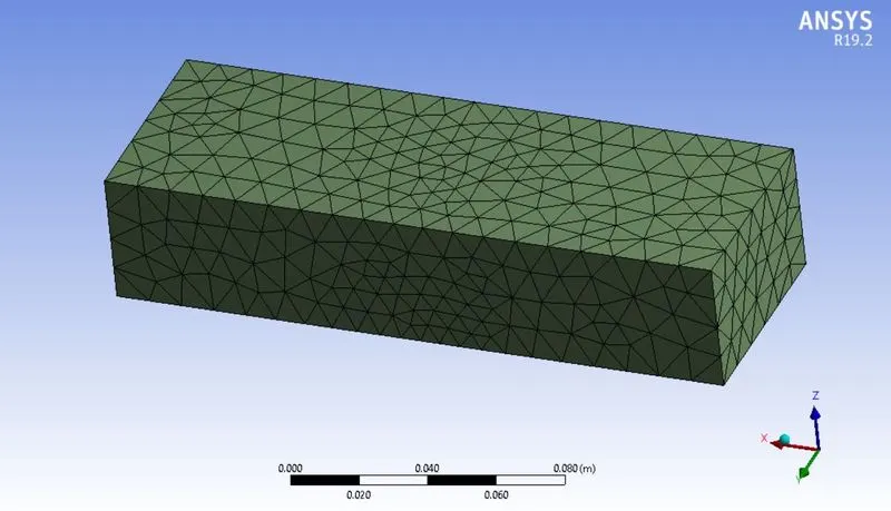
Refined Mesh:
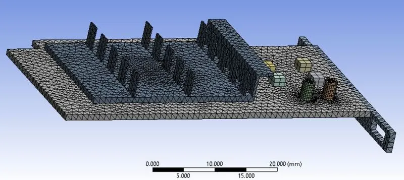
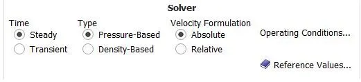
Then go to the setup option. Select the steady state -pressure -K-omega_sst type solver to solve thi simulation.
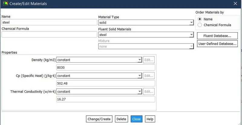
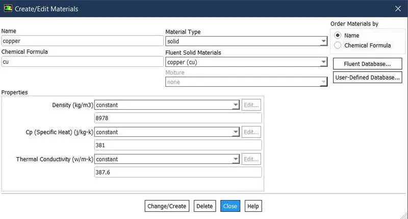
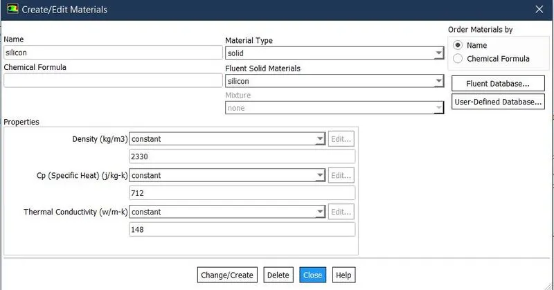
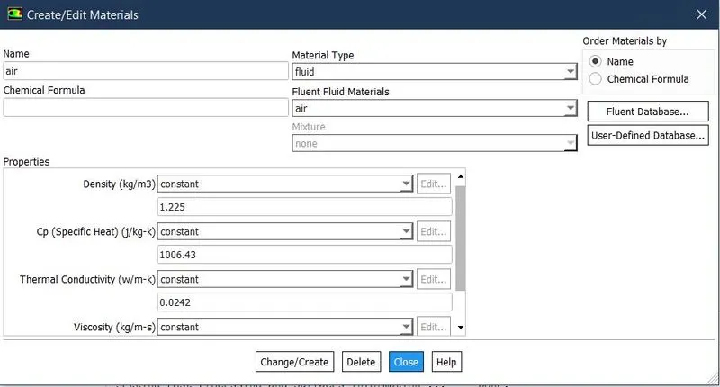
Then Add/create a required material.Then assign appropriate material to the components.
| Components | Material |
| Base | Steel |
| Fins | Copper |
| Processor | Sillicon |
| Enclosure | Air |
i) Base -Steel:
ii) Fins - Copper:
ii) Processor-Silicon:
iv) Enclosure-Air:
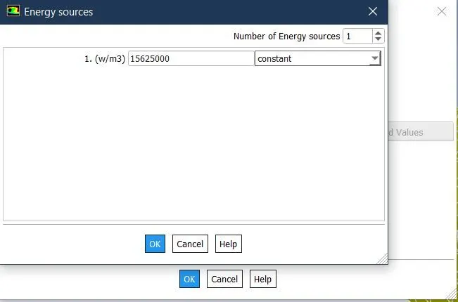
For this case consider that, our processor is a source terms and it generating heat.
So, for setting up the source term go to Zones - Cell zones - and click on the processor for editing which is in the Solid.
After that select the material to gold and click on the source terms to enabled it and set the energy source to 1.
Enter the boundary condition then initialize the simulation. Then change the iteration number then run the simulation.
After the simulation done go to the post processing process to get the required results.
Results:
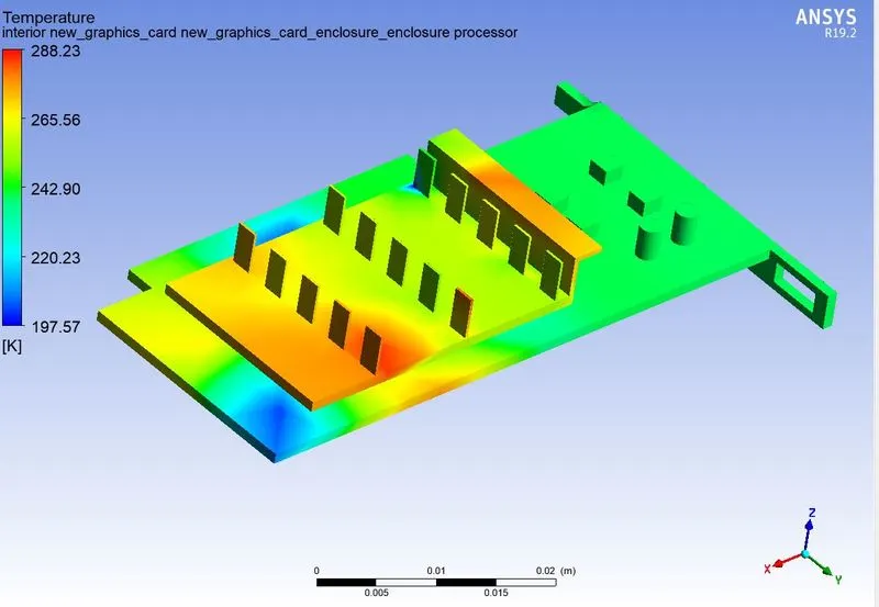
Baseline mesh:
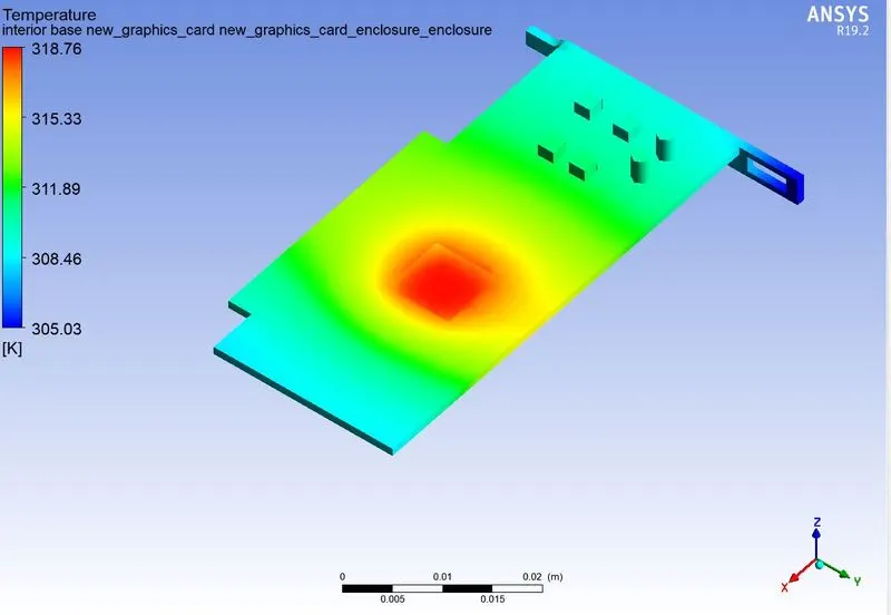
Temperature distribution:
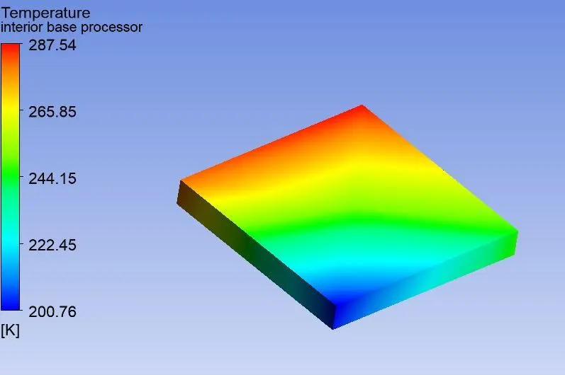
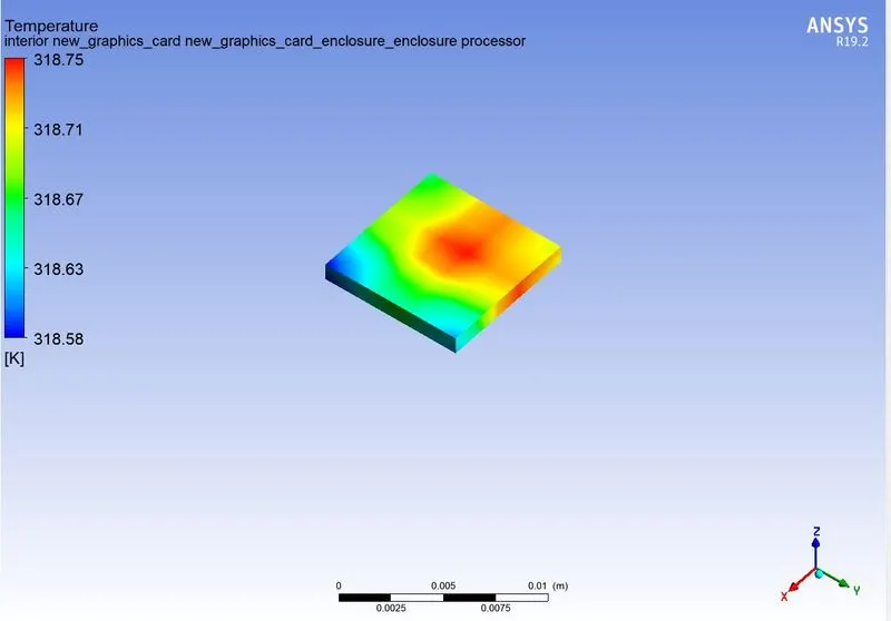
Temperature distribution at microprocessor:
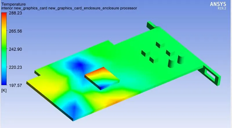
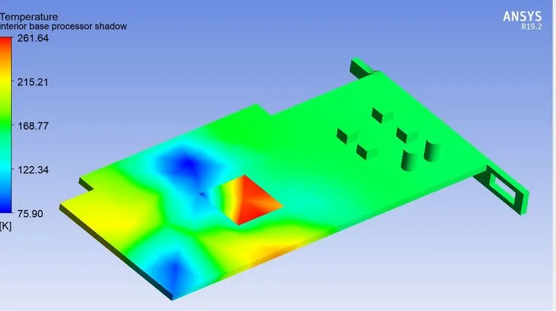
Hotspot of the model:
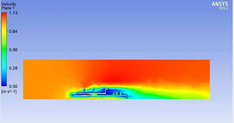
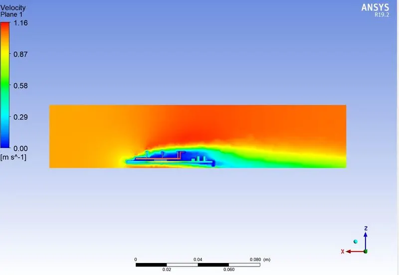
Velocity distribution:
Refined mesh:
i) Velocity = 1m/sec
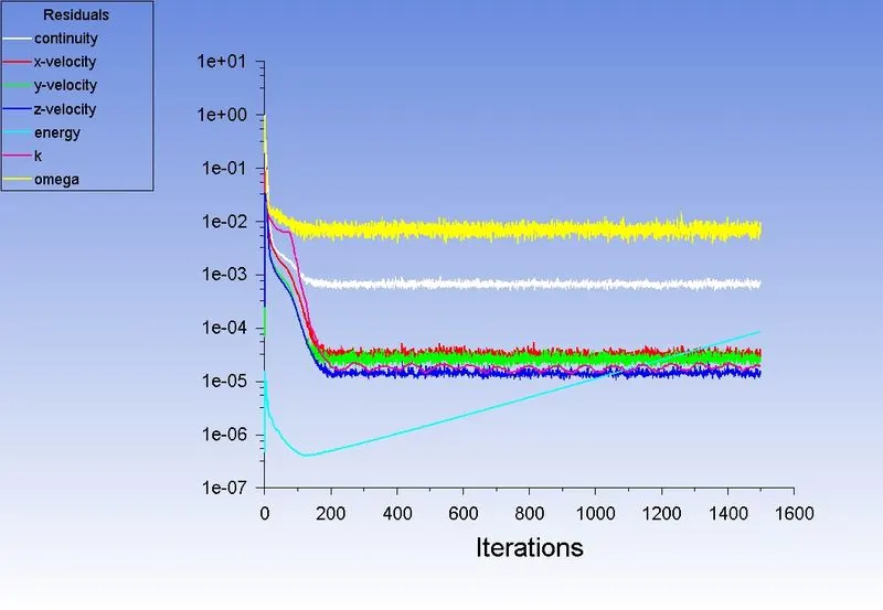
Residual:
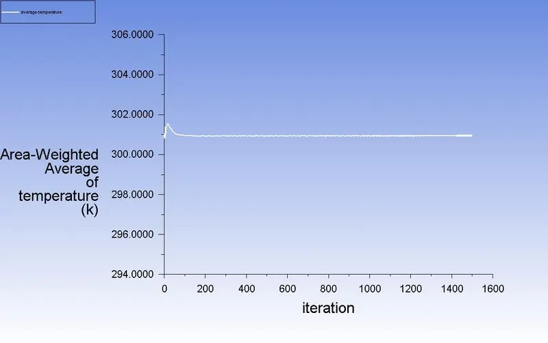
Average Temperature Distribution plot:
Temperature distribution:
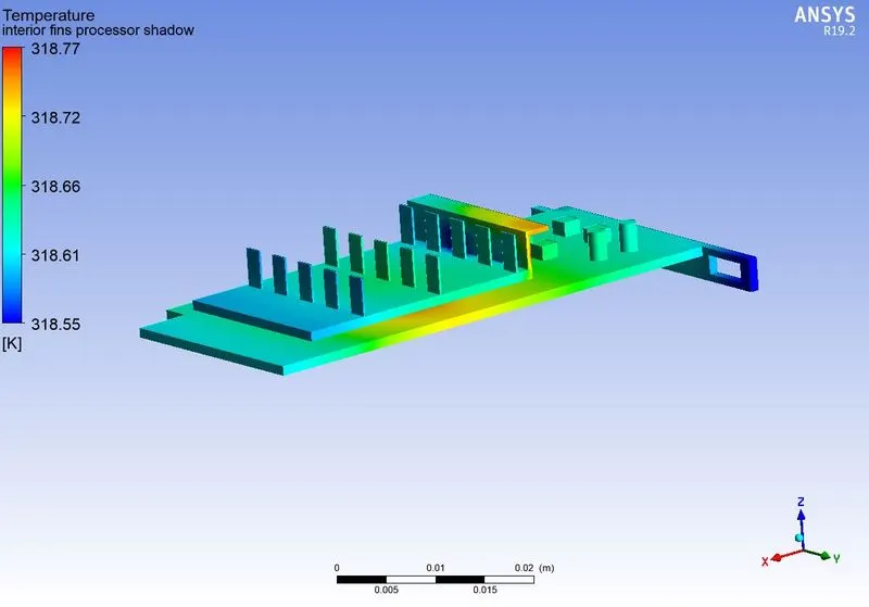
Temperature distribution at microprocessor:
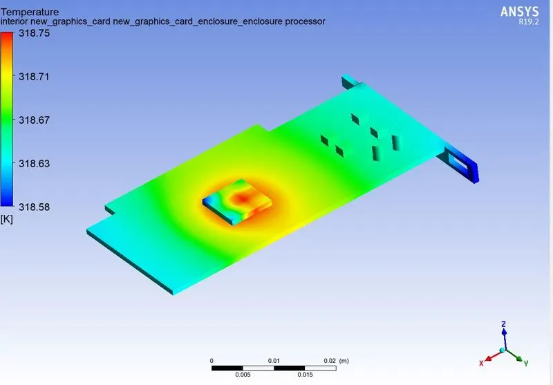
Hotspot of the model:
Velocity distribution:
i) Velocity = 2.5m/sec
Residual:
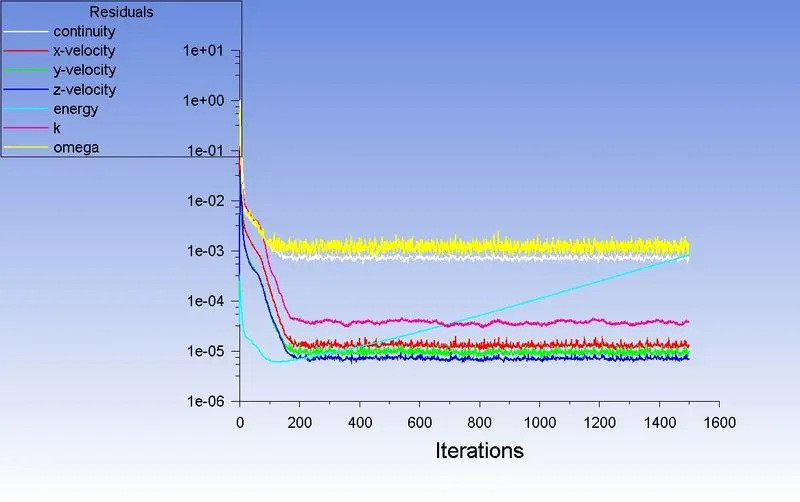
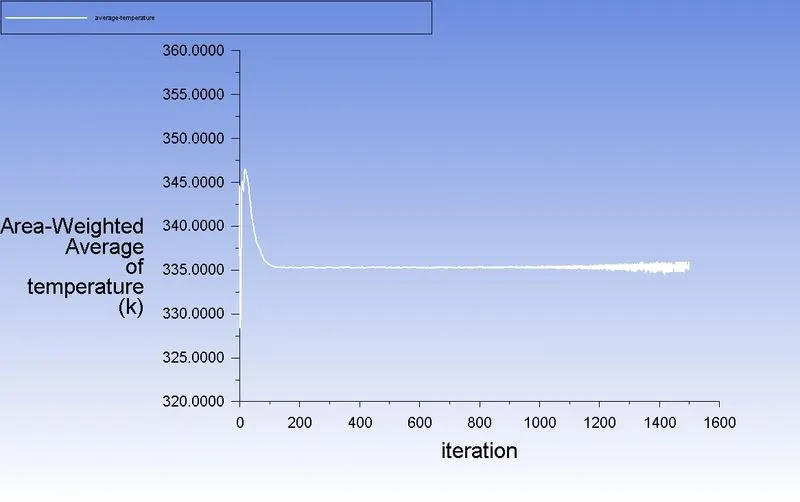
Average Temperature Distribution plot:
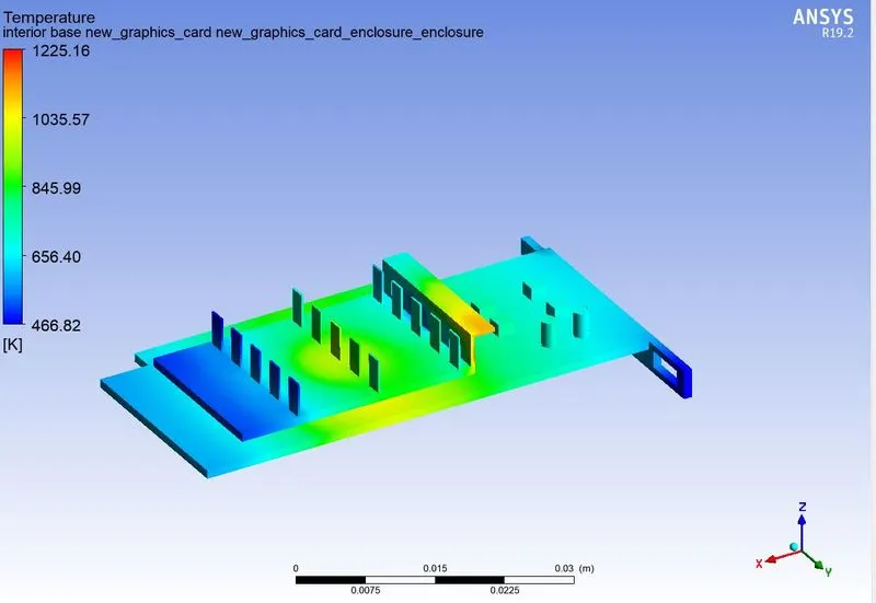
Temperature distribution:
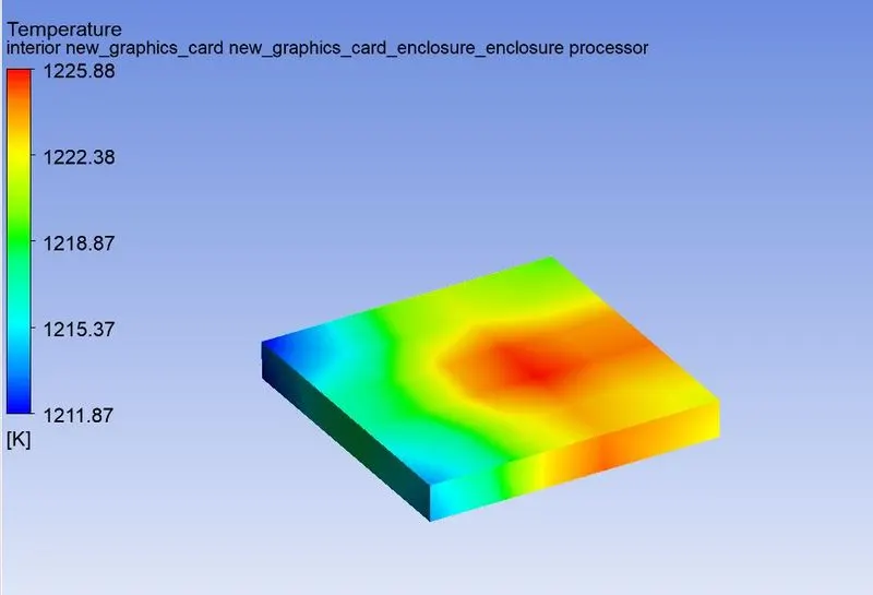
Temperature distribution at microprocessor:
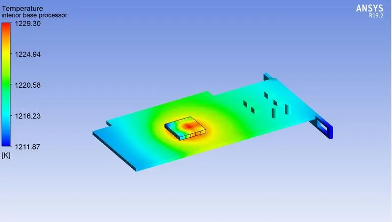
Hotspot of the model:
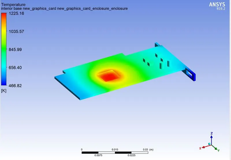
Velocity distribution:
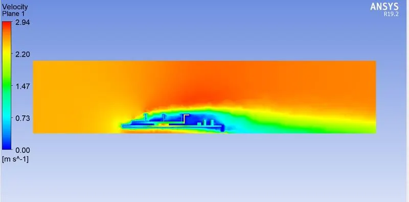
i) Velocity = 5m/sec
Residual:
Average Temperature Distribution plot:
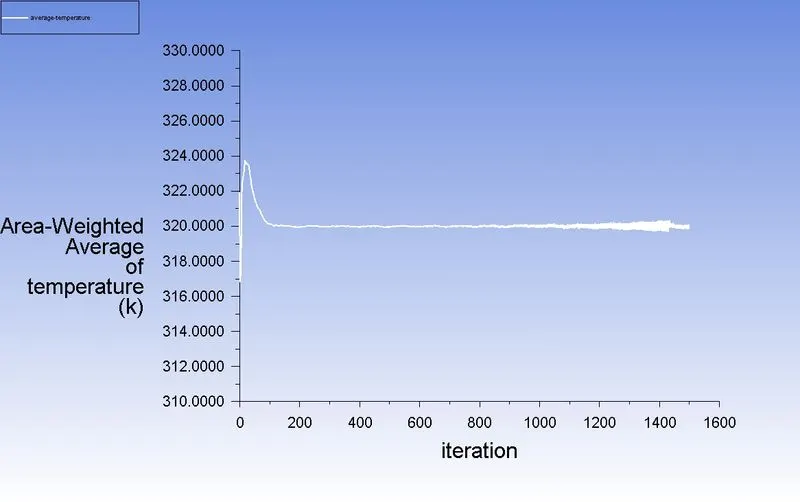
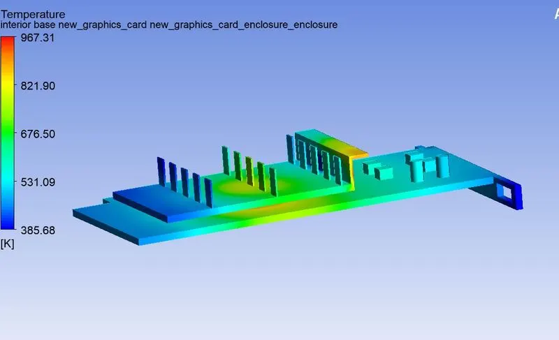
Temperature distribution:
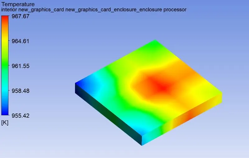
Temperature distribution at microprocessor:
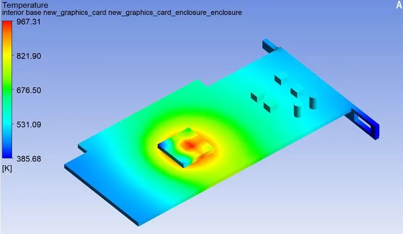
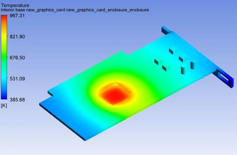
Hotspot of the model:
Velocity distribution: