Week 6 - CHT Analysis on a Graphics card

Aim:

Perform steady-state conjugate heat transfer analysis on a model of a graphics card.

Objectives:

1. Run the simulation for velocity v=1 m/s, 3 m/s and 5 m/s
2. Find maximum temperature and convective heat transfer coefficient attained by the processor
3. achieve convergence
4. identify potential hotspots on the model

Introduction:

Graphics Card:  

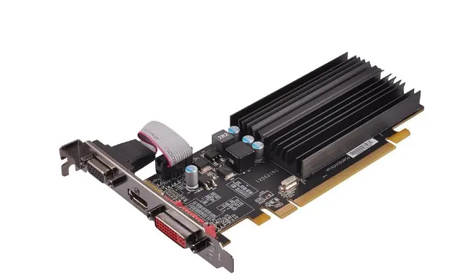
Figure: Physical model of graphics card

The graphics card is kept inside an enclosure through which air flows. the graphics card is made of multiple solid components. GPU of graphics card generates heat. the processor(Heat source) is in contact with PCB and heat sink. heat is conducted to the fins of the heat sink. fins of heat sink increase the effective area of convective heat transfer. forced convection occurs to transfer heat from fins to fluid for three different velocities. 

PCB (printed circuit board) is a non-conductive material with a conductive line printed or etched. electronic components are mounted on the board and the traces connect the components together to form a working circuit or assembly. 

PCB generally consists of four layers, which are heat laminated together into a single layer. The different types of PCB materials used in PCB from top to bottom include Silkscreen, Soldermask, Copper and Substrate. 

The last of those layers, substrate, is made of fibreglass and is also known as FR 4, with the FR letters standing for "fire retardant." This substrate layer provides a solid foundation for PCBs, though the thickness can vary according to the uses of a given board.

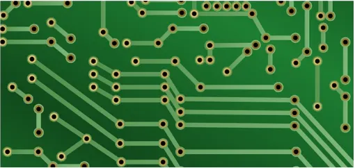
Figure: Printed circuit board (PCB)

Theory:

Conjugate Heat Transfer:

For conjugate heat transfer analysis, solid material conduction and fluid convection are analysed simultaneously. the conductive heat transfer in the solid region is coupled to convective heat transfer in neighbouring fluid flow. 

why CHT analysis is used?

•  CHT analysis allows simulating heat transfer between solid domain and fluid domain by exchanging thermal energy at the interface between them. 

•  the contemporary conjugate convective heat transfer model was developed after computers came into wide use to substitute the empirical relation of proportionality of heat flux to temperature difference with heat transfer coefficient which was the only tool in theoretical heat convection since the times of Newton.

•  This CHT model, based on a strictly mathematically stated problem, describe the heat transfer between a solid body and flowing fluid over the body or inside the body. the physical processes and the solutions of governing equation are considered separately for each object in two subdomains(Fluid domain and solid domain). matching conditions of these solutions at the interface provides the temperature distribution and heat flux(q) along with the fluid body interface, eliminating the need for heat transfer coefficient(h).

• CFD solver solves the fluid flow along with the energy equation for the fluid and solid. conjugate heat transfer by using a CFD solver directly solves the heat transfer between solid and fluid. hence there is no need to define convective heat transfer coefficient(h). 

• However, we can easily calculate the convective heat transfer coefficient (h) which is a key unknown in convective heat transfer by using the conjugate heat transfer approach performs in the CFD solver. 

Baseline Simulation steps:

1. Geometry
2. Mesh
3. Setup
4. Solution
5. Result

Step 1: Geometry

we do uncheck the components one by one to see each and every component of the Graphics card.

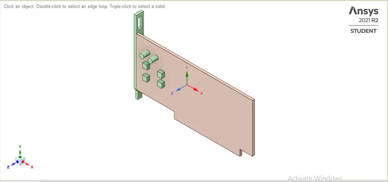
Figure 1.1: Base components (Capacitors, Transistors)

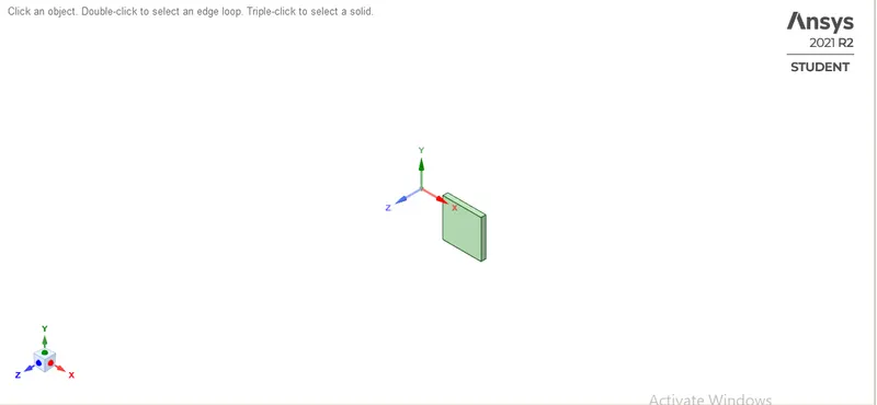
Figure 1.2: Processor / Heat Source

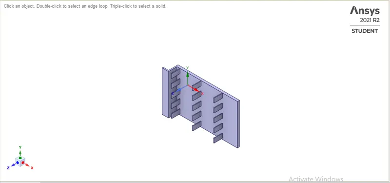
Figure 1.3: Fins / Heat Sink

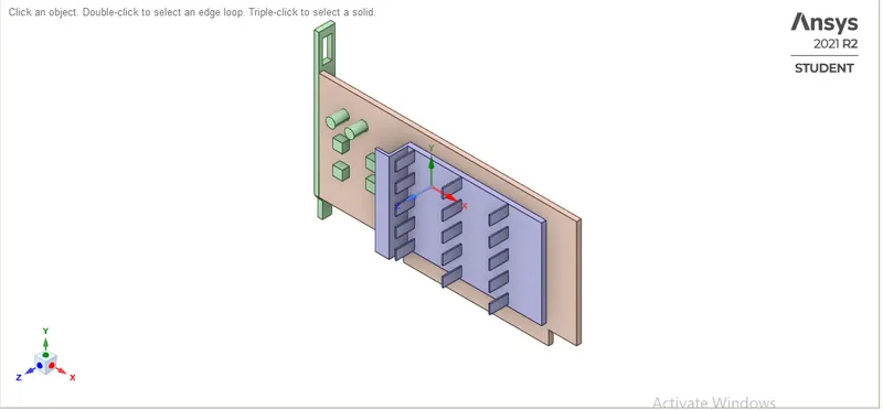
Figure 1.4: Graphics Card

Now we do share topology(faces, edges, vortex connections) between touching or intersecting bodies and surfaces. 

 

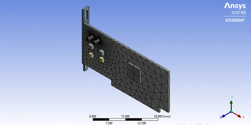
Figure 1.5:  Shared Topology

Step 2: Mesh: 

basic mesh is generated using the standard value(element size is by Default) in Ansys. this mesh is used to obtain an initial solution which will help to identify the locations where mesh refinement is required. 

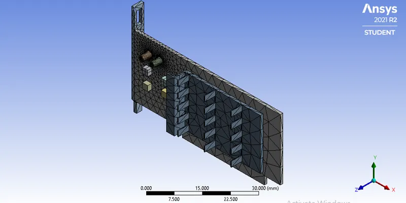
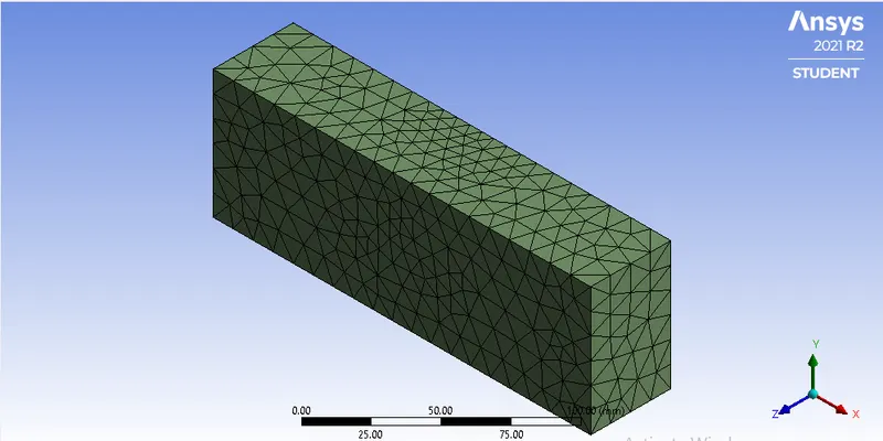
Figure 2.1: Mesh

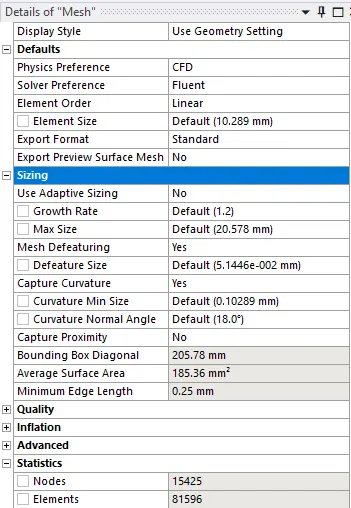
Figure 2.2: Mesh details

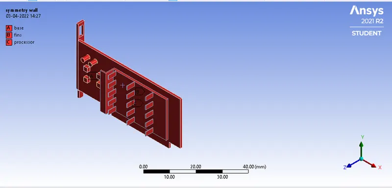
Figure 2.3(a):  Named selection

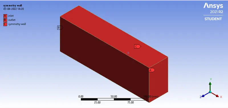
Figure 2.3(b): Named Selection

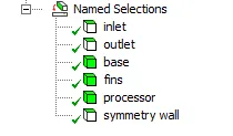
Figure2.3(c): Complete Named Selection

Step3: Setup

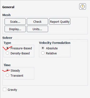
Figure 3.1: Solver selection

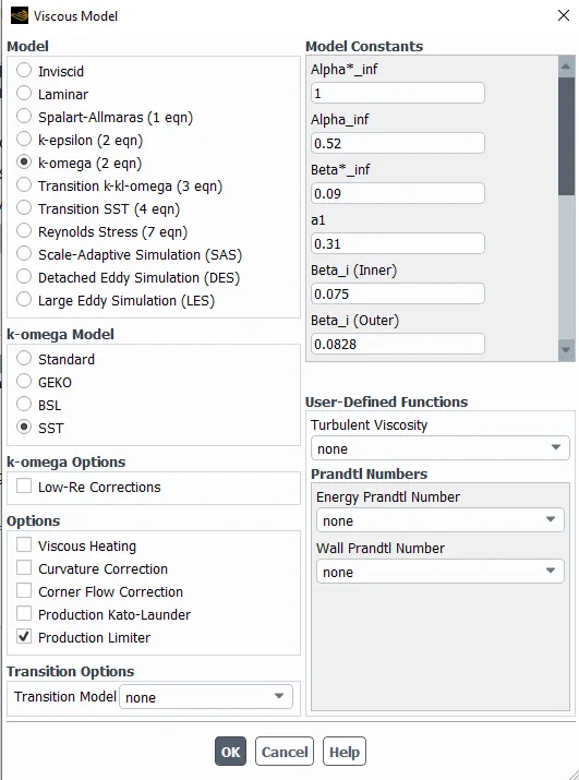
Figure 3.2: Turbulent Model Selection and turn on Energy Tab. 

Material Properties:

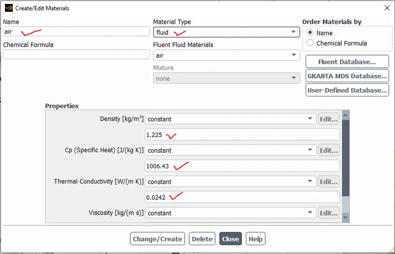
Figure 3.3: Air properties

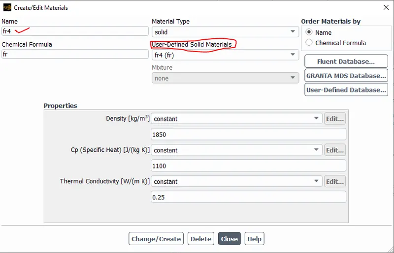
Figure3.4: properties of printed_circuit_board/PCB which is made of fr4

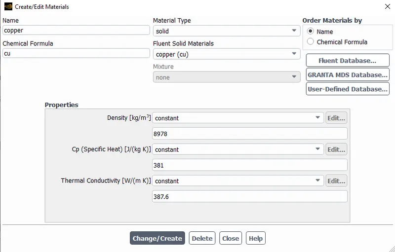
Figure 3.6: Copper properties

Cell Zone Conditions:

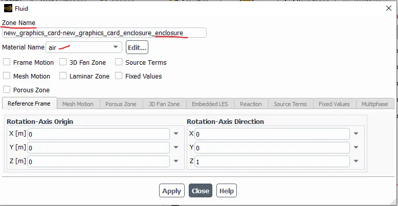
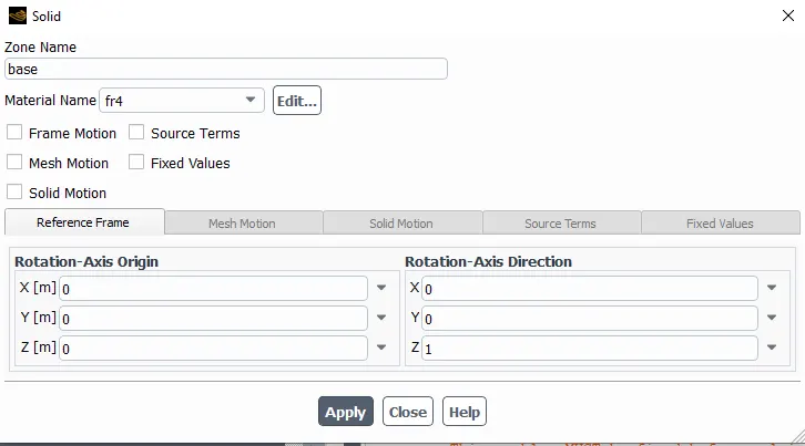
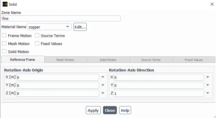
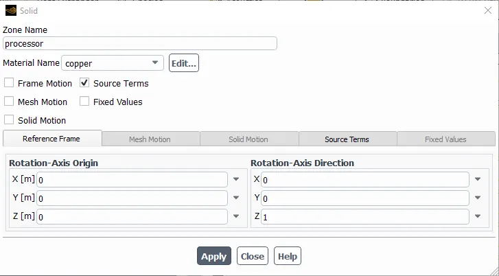
volume of processor=`8mmtimes8mm times1mm=64 mm^3=64times10^-9 m^3`

consider NVIDIA GT 730 graphics card, its thermal design point i.e. the amount of heat generated by the processor which is to be dissipated by the heat sink(fins) is 49 watts. so heat generation rate =`202148437.5 W/m^3`

Convergence:

I gave 500number of iterations to run the simulation. but the solution is converged at 95 iterations.

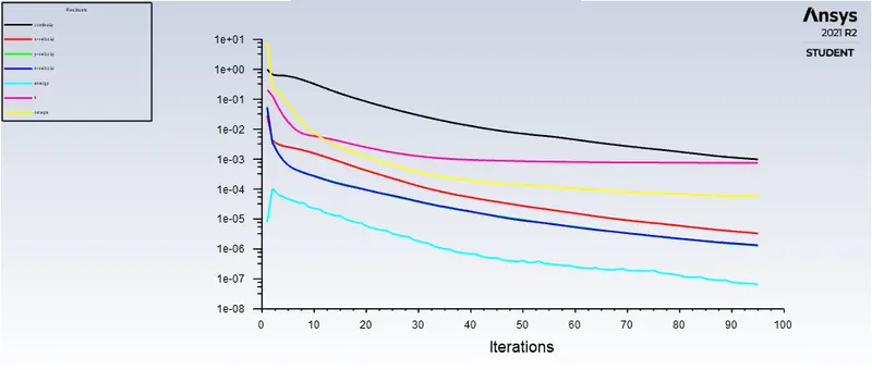
Figure: Residuals plot

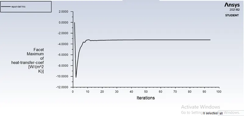
Figure: Maximum heat transfer coefficient plot

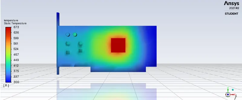
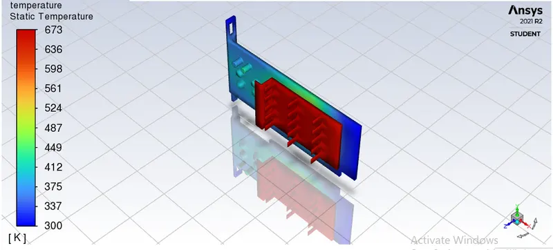
Result:

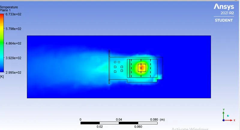
 Figure: Temperature contour

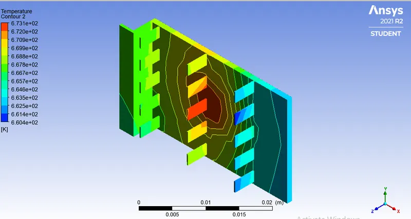
Figure: Temperature contour at fins

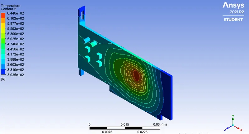
 Figure: Temperature contour  at base

Hotspot: 

the maximum temperature (hotspot) is at the interface of the processor and fin base. so it requires further refinement of mesh for accurate analysis. hence in the case of refinement (case 2), we reduce the mesh element size of the processor and fins by using body sizing command. 

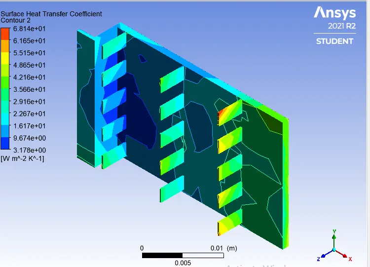
Figure: contour of HTC at fins

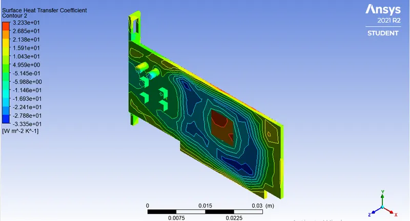
Figure: Contour of HTC at base

Caes 1: Refined mesh(V=1 m/s)

• 2Refine Mesh: 

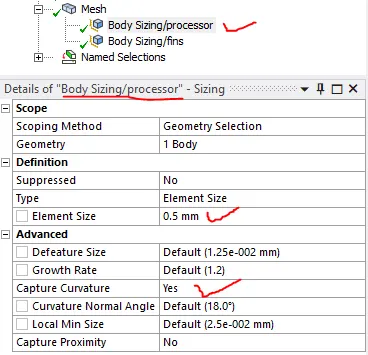
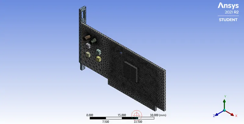
Figure:  Mesh refinement on the processor 

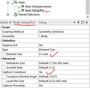
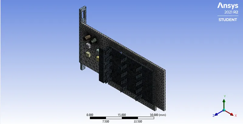
Figure:  Mesh refinement on the fins

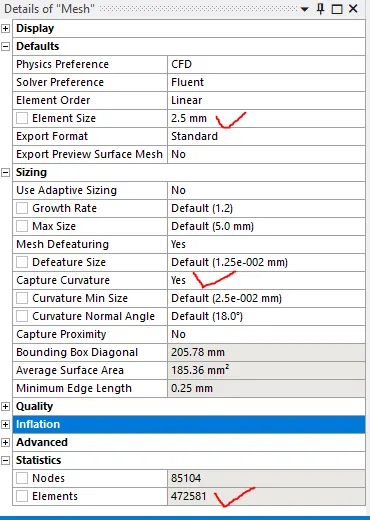
Figure: Mesh details

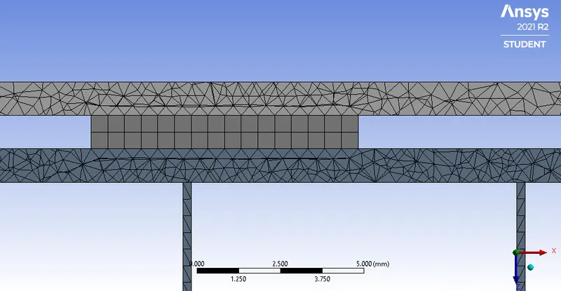
Figure: Cut section view 

Setup / solution:

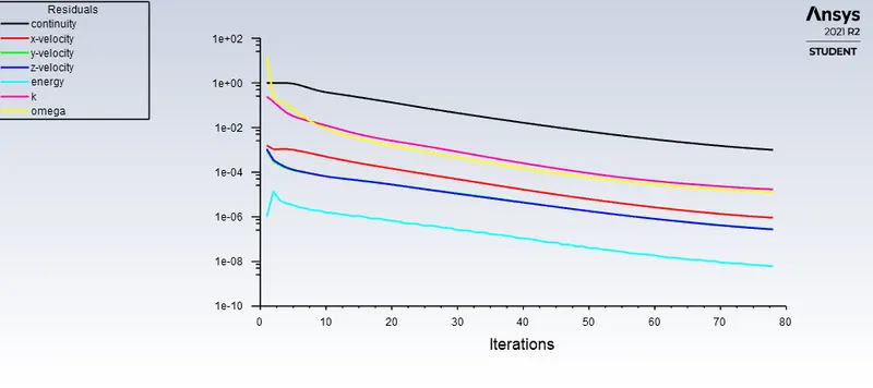
Figure: Residual plot 

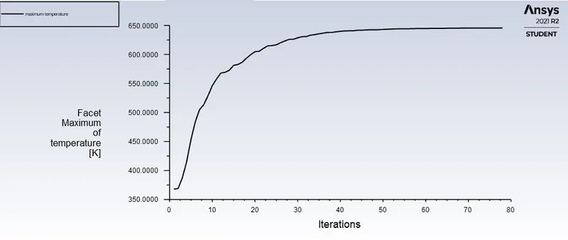
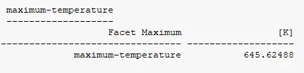
Figure: Maximum temperature 

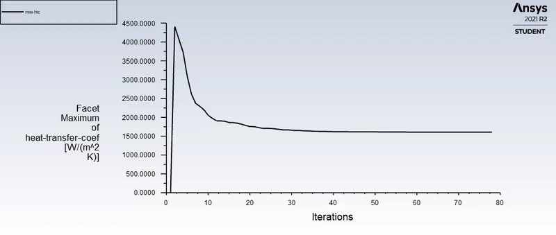
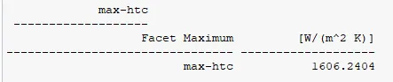
Figure: Maximum HTC

Result: 

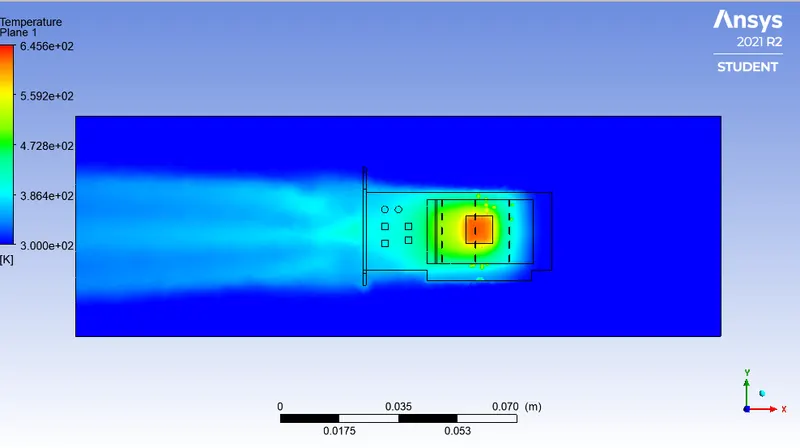
Case 2: (V=2 m/s)

 

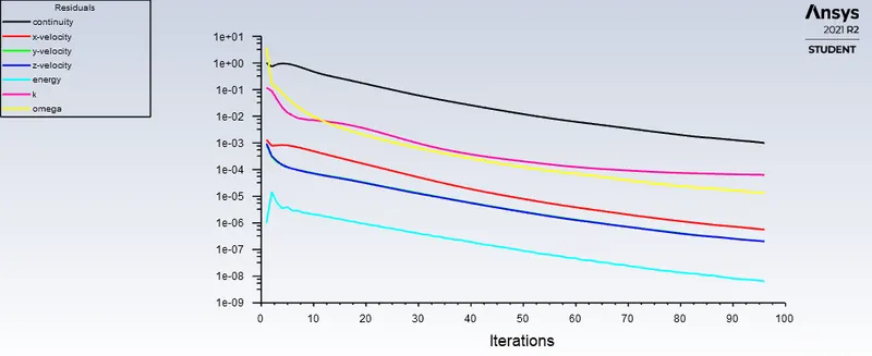
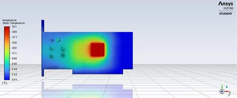
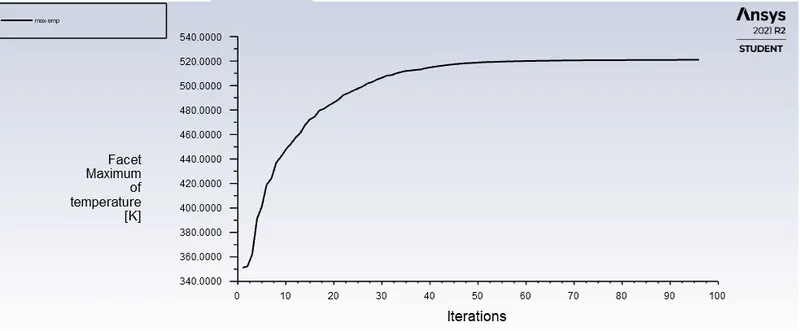
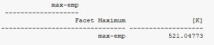
 Figure: Maximum temperature plot

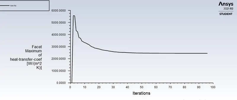
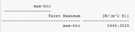
Figure: Maximum HTC

Summary:

Case	Velocity (m/s)	Convergence iteration	Maximum temperature (K)	Maximum Heat transfer coefficient (W/m2K)
Baseline simulation	1	94	673.07599	-3.230633
Refinement	1	78	645.62488	1606.2404
	2	73	521.04773	2446.3525