Week 6 - CHT Analysis on a Graphics card
Aim: To perform CHT analysis on Graphics card.
Objectives:
- Perform Simulations by varying the velocity from 1 to 5 m/s for a minimum of 3 values.
- Find the Max Temperature and Heat Transfer Coefficient of the system
- Prove Convergence of the simulation by using plots and graphs.
- Identify hotspots on the object.
Theory:
CHT stands for Conjugate Heat Transfer Analysis. This type of analysis allows for simulation of heat transfer between Solids and Fluids by an interchange of thermal energy at its interfaces.
CHT analysis is used to create simulations of heat exchangers, cooling of electronic equipment and general-purpose air-conditioning devices
They are also used in determining the outcomes of
- Heat Transfer coefficient Analysis
- Heat Flux analysis
- CFD Thermal Analysis
- Temperature Distribution Analysis
There are three contributions to heat transmission due to fluid motion:
- The downloaded geometry is edited in Spaceclaim
- The option 'Share' is used to attain conformal mesh between the components.
- Share topology is to be enabled so that the necessary information can be transferred between the cell-zones.
Mesh Setup:
- All the components are to named, so it is easy to setup in Fluent.
- Body sizing is to be applied to each and every named selection to obtain proper meshing.
- Baseline mesh is generated, which is to have hundred thousand elements to have an accurate solution.
- After mesh is setup, exit 'Meshing' to open Fluent.
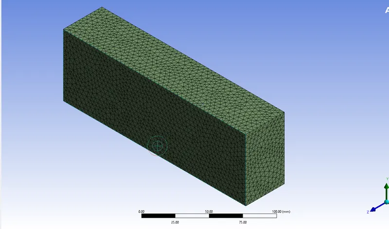
Enclosure.
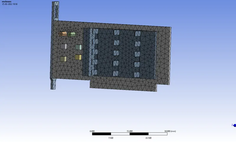
Graphic card setup.
Base.
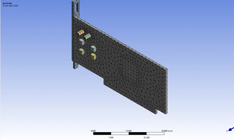
Processor.
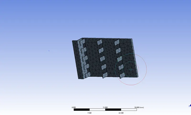
Fins.
Fluent Setup:
This experiment is conducted on Fluent.
Setting up Physics for CHT analysis on Fluent.
- Steady-state, Pressure based Solver.
- Absolute velocity.
- Energy equations are used
- Viscous K-omega Model is used.
Materials:
Materials for each named selection is shown in the dialog box below.
|
Name |
Density (kg/m^3) | Specific Heat(J/kg-K) | Thermal Conductivity(W/m-K) |
|
Copper |
8978 | 381 | 387.86 |
|
Silica |
2328 | 710 | 150 |
|
Steel |
8050 | 502 | 16.27 |
Air is used used as fluid medium.
Density:1.225 kg/m^3
Viscosity: 1.7894e-05 kg/ms
Setting Up Source Terms:
- In this case, Processor is a source of heat. So, we have to assign a value of heat generated by the processor through 'Source terms' option.
- to setup source terms, Go to Cell-zone conditions-processor and enable source terms.
Step-1: Baseline Mesh:
Velocity: 1m/s
Mesh:
Enclosure: 3.9mm
Fins: 2 mm
Processor: 1.5 mm
Base: 2 mm
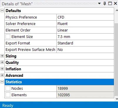
Mesh Details.
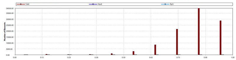
Mesh Metrics.
Enclosure and Graphic card:
Enclosure.
Graphic card setup.
Base.
Processor.
Fins.
Step-1: Refined:
Velocity: 1m/s
Mesh:
Enclosure: 2.5mm
Fins: 0.75 mm
Processor: 0.5 mm
Base: 0.75 mm
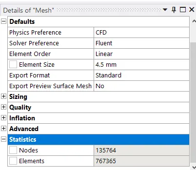 Element details
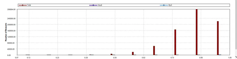
Mesh Metrics
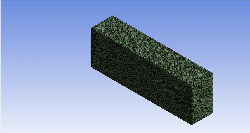
enclosure
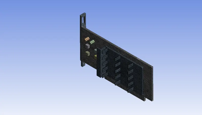
Fins
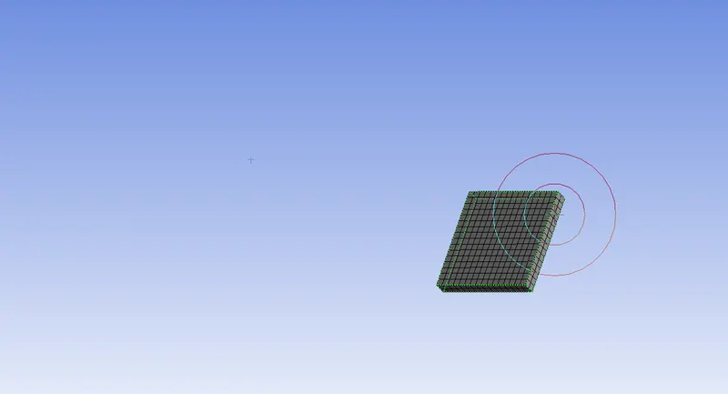
Processor
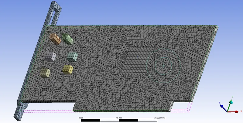
Base plate.
Baseline mesh analysis:
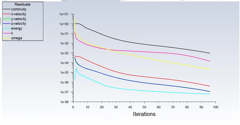
Residuals
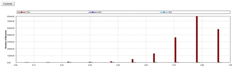 Mesh metrics
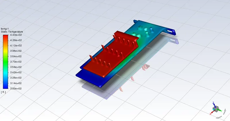 Solution animation
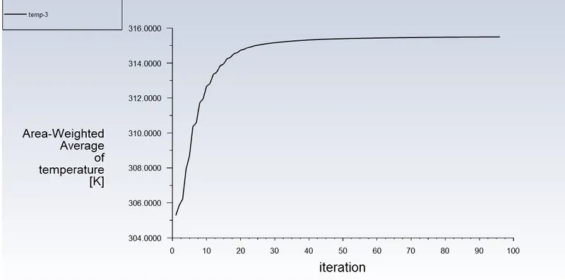 Weighted average of Temperature
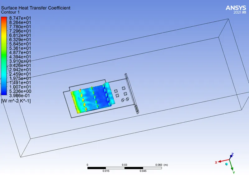 Heat Transfer coefficient
 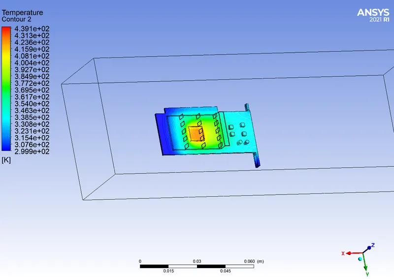 Hotspots on the Base
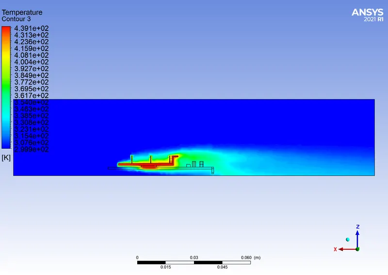
Refined mesh Case-1:
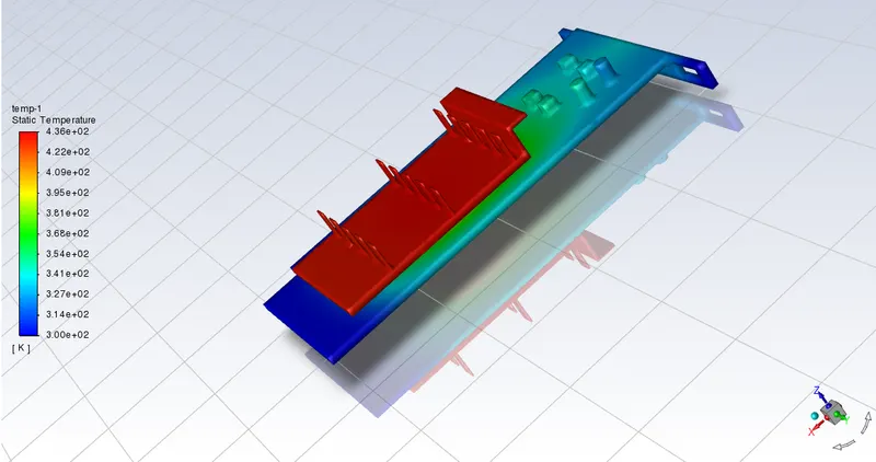 Solution Animation
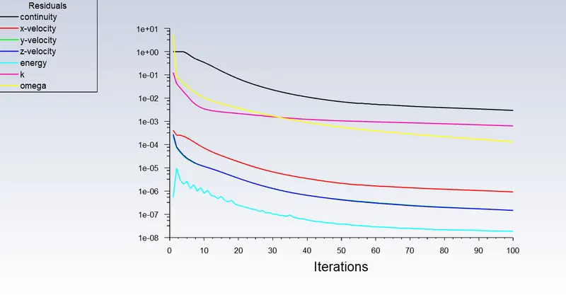 Residuals
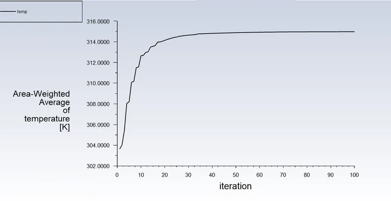 Weighted Average of Temperature
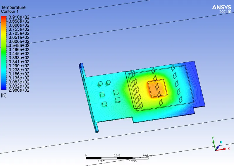 Hotspot on the Base
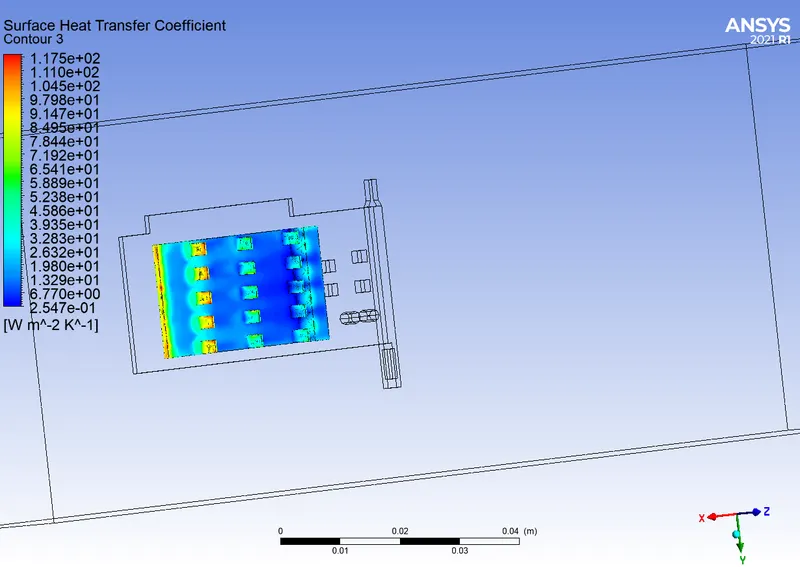 Heat transfer Coefficient
 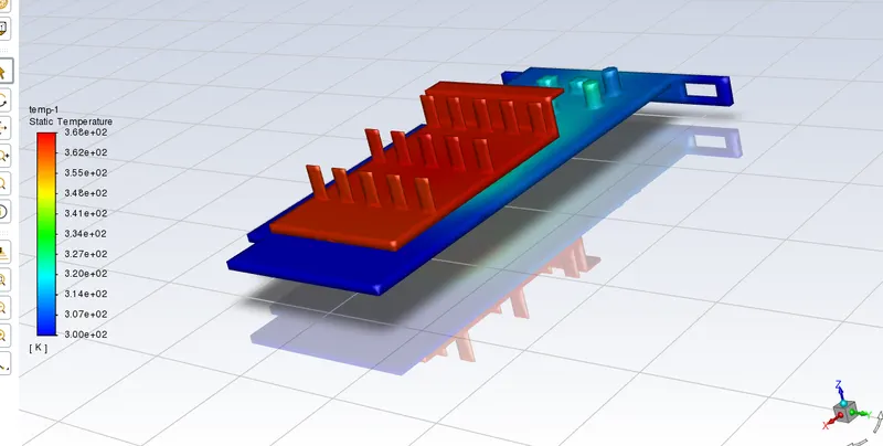 Solution Animation
 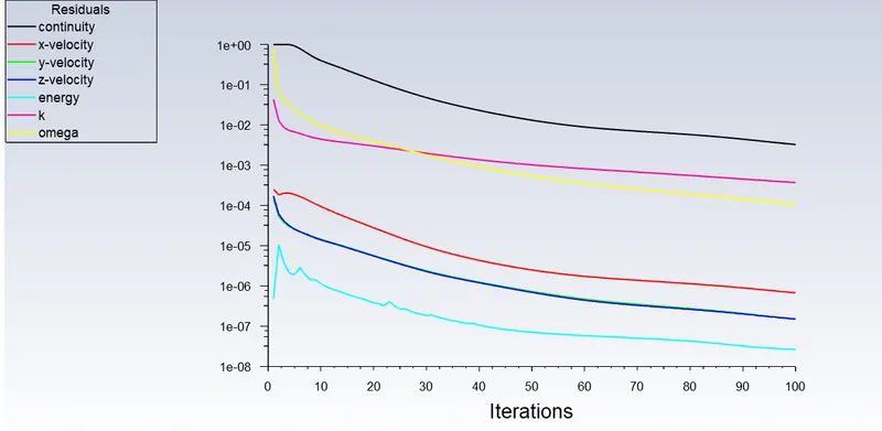 Residuals
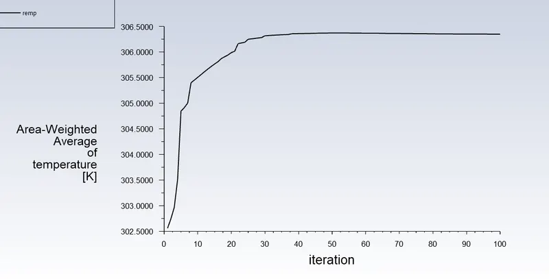 Weighted average of Temperature
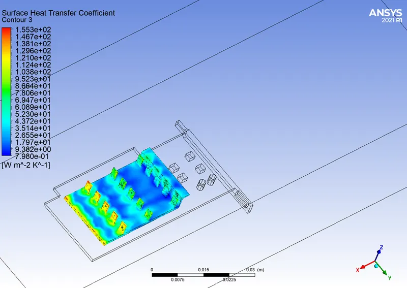 Heat transfer Coefficient
 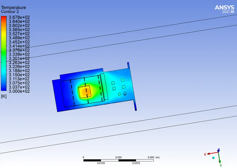 Hotspots on Base
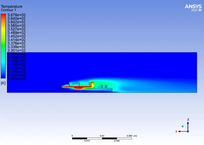 Temperature Contour
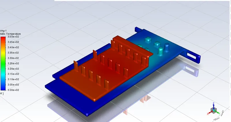 Solution Animation
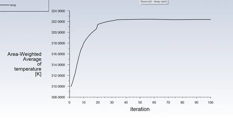 ResidualsWeighted Average of Temperature
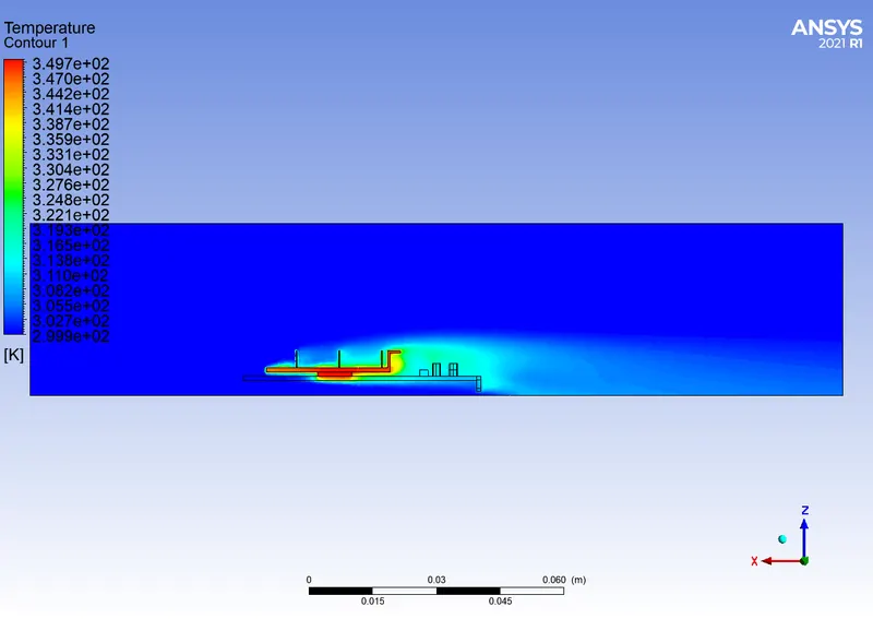 Temperature Contour
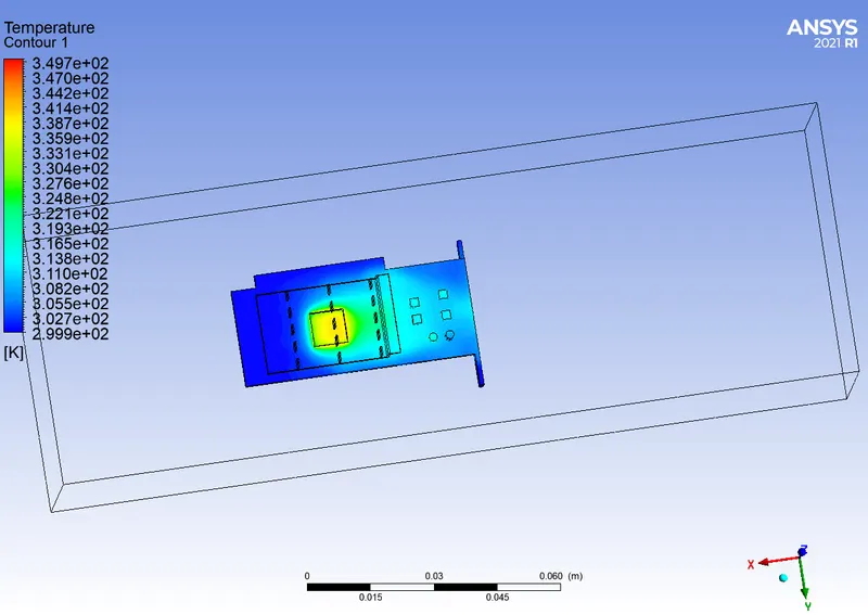 Hotspots on Base
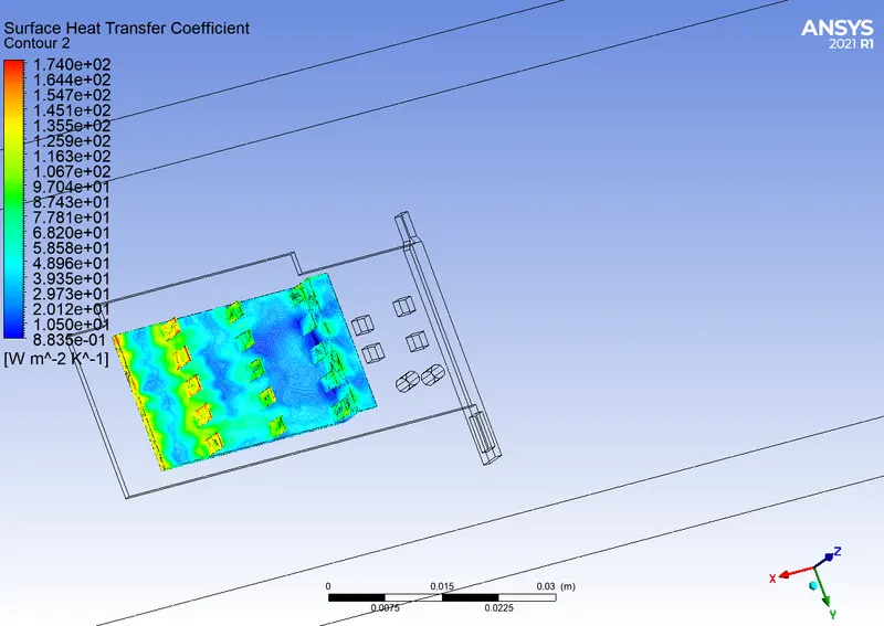 Heat Transfer Coefficient
| Baseline, V=1m/sec | Refined,V=1 | Refined,V=3 | Refined,V=5 | |
| Heat Transfer Coefficient | 88.2805 | 118.814 | 156.748 | 175.576 |
| Max Temperature | 440.349 | 391.836 | 323.569 | 350.21 |