Week 5 - Rayleigh Taylor Instability
Aim: To conduct the Rayleigh Taylor Instability CFD simulation.
Indroduction: Rayleigh Taylor Instability occurs at the interface of fluids with different densities. The less denser fluid pushes the more dense fluid in an attempt to reduce its combined Potential Energy.
Theory: The early disruptions of the RT instability shift from a linear to a non-linear development phase as the RT instability develops, eventually forming "plumes" flowing upwards and "spikes" dropping downwards. The fluid flow may be closely approximated by linear equations in the linear phase, and the magnitude of perturbations increases exponentially with time. The perturbation amplitude is too great for a linear approximation in the non-linear phase, hence non-linear equations must be used to describe fluid dynamics. The structure of following non-linear RT instability flows is often determined by the density discrepancy between the fluids.
Examples include Mushroom cloud on volcanic Eruption, Supernova, Water atop oil.
Practical CFD models that are based on the Rayleigh Taylor waves.
1. Mass diffusion model:
The mass diffusion equation represents how viscosity promotes mass and energy movement and mixing in fluids. I if any configuration is Rayleigh-Taylor unstable, if the viscosity is high enough, the diffusion mechanism may cause substantial mixing.
2. Single fluid model:
2.1. Potential flow model
This model applies for all stages of instability from linear to early non-linear to asymptotic, though it's confined to Atwood number = 1. Single-mode perturbation in this model raises the flow equations to second order around the bubble tips, yielding an ordinary differential equation for the bubble velocity.
2.2. Buoyancy drag model
It's true for any Atwood number, but only for non-linear stages of the instability. The breadth of the mixing layer is changed using ordinary differential equations. The amplitudes of bubbles, or spikes, are characterised by balancing the forces of inertia, buoyancy, and drag. These models are unable to describe numerous mixing interfaces, are difficult to expand to two or three dimensions, and, in most cases, do not handle demixing, also known as counter gradient transport, which is the reduction of total fluid masses inside the mixing zone. Two-fluid (or multi-fluid)models must be utilised to solve the challenges mentioned above.
2.3. Besnard-Harlow-Rauenzahn(BHR)
It's an improved version of the single-fluid model. The evolution equations coming from second-order correlations and gradient-diffusion approximations form the basis of the BHR model. The original BHR model includes comprehensive transport equations for the Reynold stresses, turbulent mass-flux velocity, density fluctuations, and the turbulent kinetic energy dissipation rate using a mass-weighted averaged decomposition.
3. Multi-Fluid model:
These models, in addition to the original flow equations, utilize an unique system of equations for each fluid and enable an accurate modelling approach for demixing by accurately capturing the relative velocity of the distinct fluid components.
Reynold averaging of governing equations and consequent terms is the initiation phase in the formulation of turbulence models.
3.1. Two equation K-L turbulence model:
Formulae describing turbulent kinetic energy, K and turbulent length scale, L are used in K-L turbulence model. The buoyancy-drag equations for the self-similar emergence of RT instabilities are being used to generate the model equations.
3.2. Three-equation K-L-a turbulence model:
The three-equation model was created as an extension of the two-equation K-L model, including a third equation for turbulent mass-flux velocity.
3.3. Four-equation K-L-a-b turbulence model:
A fourth equation for density-specific volume covariance was introduced to the three-equation K-L process to improve the four-equation model. The effects of alterations in density fluctuations can be accurately portrayed by model.
Modelling Approach:
Pre-Processing:
Step-1:Geometry
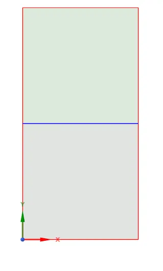
The geometry is 2 squares over each other, with a side of 20 mm. the top square is for 'water' and lower is for 'air'. the common surface is shared using the 'share to workbench' option.
Step 2: Meshing:
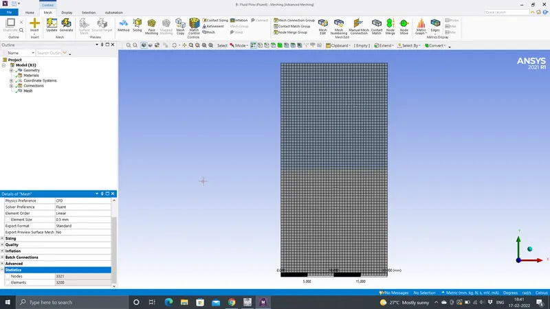
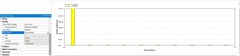
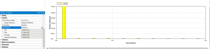
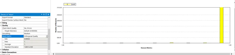
I. Baseline Mesh:
Mesh size:0.5mm
Nodes:3321
Elements:3320
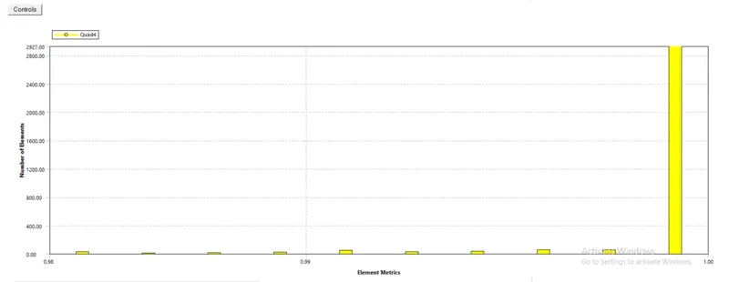
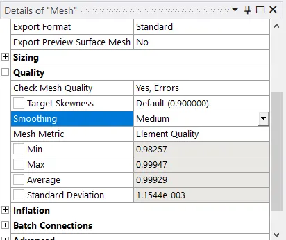
1. Element Quality
2. Aspect Ratio
3. Skewness
4. Orthogonal Quality
II. Refined Mesh
Mesh size:0.2mm
Nodes:20301
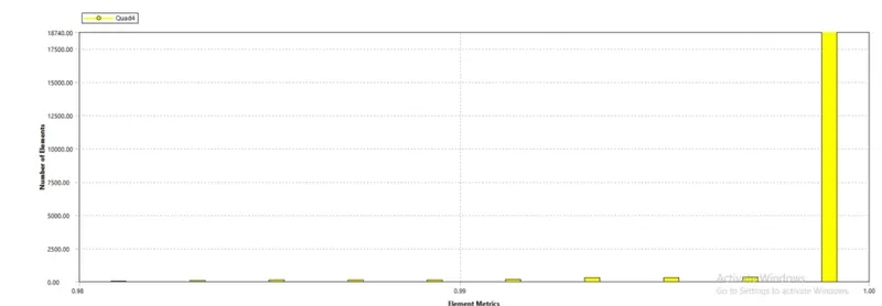
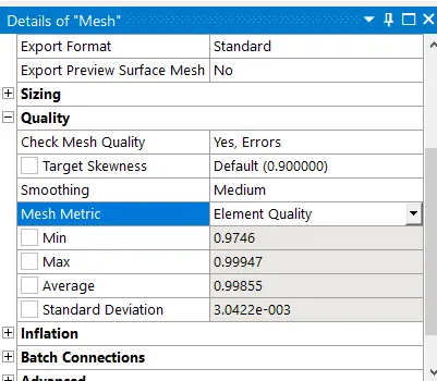
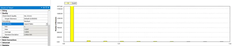
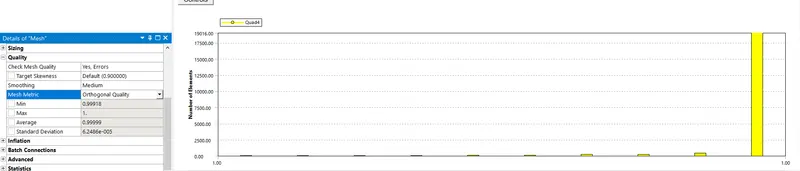
Elements:20000
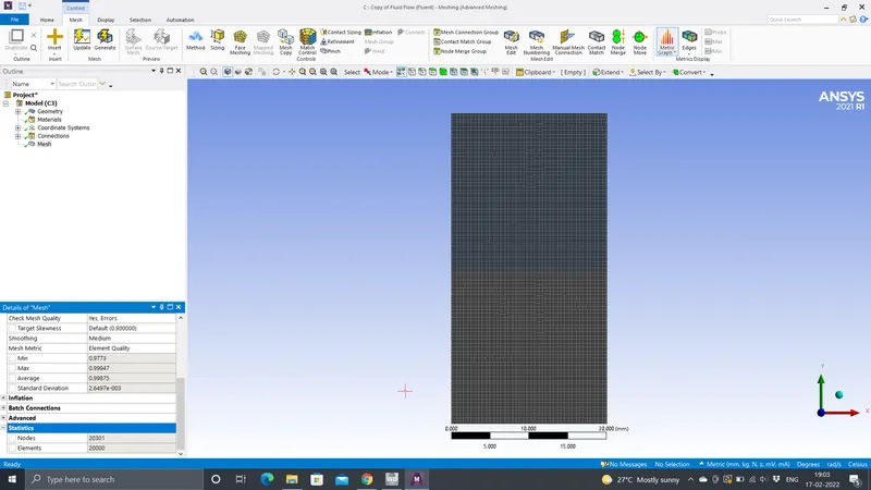
1. Element Quality
2. Aspect Ratio
3. Skewness

4. Orthogonal Quality
Step III: Fluent Settings
Pressure based, Transient Solver, Absolute Velocity @ g=9.81m/s^2, Laminar Viscous model
Material Creation And Properties:
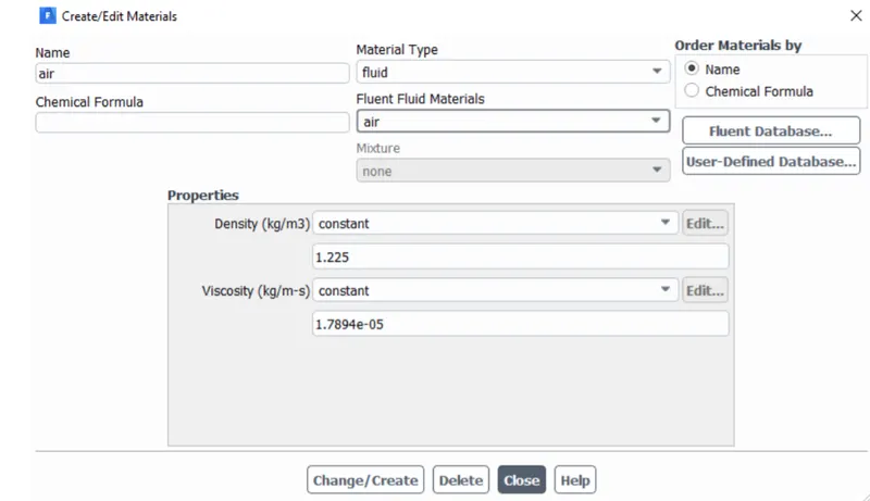
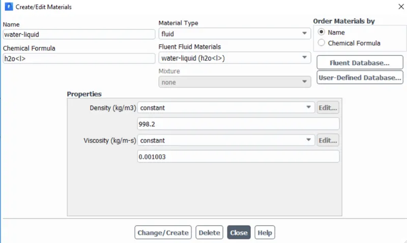
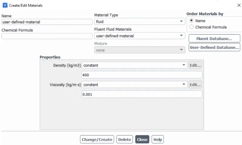
Multiphase Model:
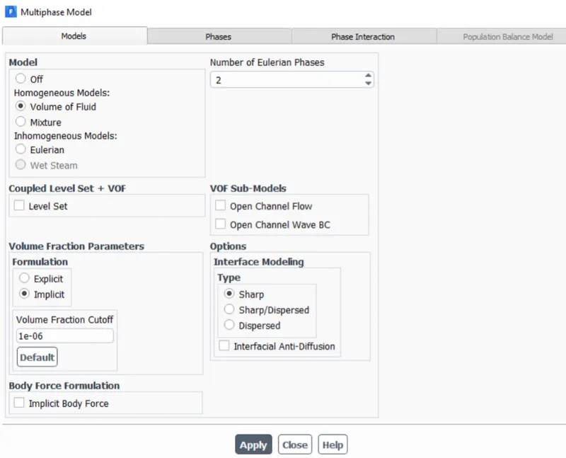
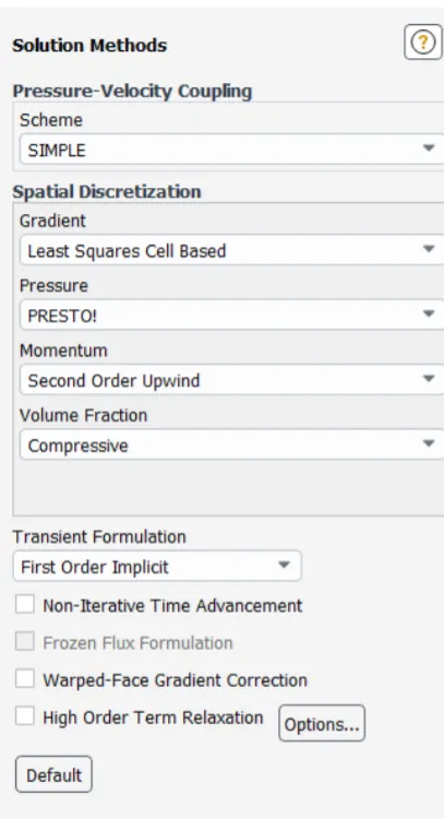
Solution Methods:
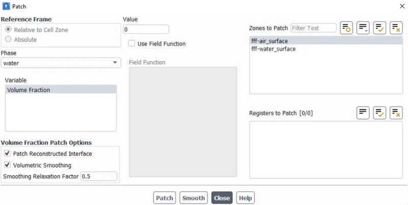
Patch:
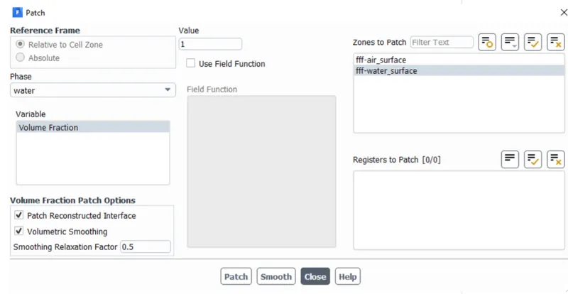
Animations:
Baseline mesh
Refined mesh
Modified case
Observations:
Finer mesh shows perfect course of the instabilities in the fluid system. But, it takes longer time than coarse mesh. results are produced accurately.
since, the instabilities are unpredictable over the course of time, transient flow is preffered.
Atwood Number:
It used to calculate hydrodynamic instabilities in density layered flows. It is dimensionless.
A =ρ1 − ρ2/ρ1 + ρ2
Where,
ρ1 is density of heavier fluid
ρ2 is density of lighter fluid
For Air-water RT instability,
ρ1= 998.2 kg/m^3 [Water density]
ρ2= 1.225 kg/m^3[Air density]
A = (998.2-1.225)/(998.2+1.225)
A = 0.998
For water- UD material RT instability,
ρ1 = 998.2 kg/m^3[Water density]
ρ2 = 1.225 kg/m^3[UD material density]
A = (998.2-400)/(998.2+400)
A = 0.428
Behaviour of RTI with change in Atwood number
Linear stability, mushroom head (falling) or bubble (rising) generation, and long-term development resulting to bubble merging and mixing are the three stages in RTI evolution. The bubble and mushroom head form is rather symmetrical for low Atwood numbers, and the disturbances or perturbations are linear over a longer duration. In contrast, with a big Atwood number, the bubble and mushroom head form is less symmetrical, and it happens at a faster pace, resulting in a non-symmetrical result.