Week 6 - CHT Analysis on a Graphics card
PROBLEM STATEMENT –
Perform a steady-state conjugate heat transfer analysis on a model of a graphics card. You can use appropriate materials of your choice for the simulation. Make sure to properly define the correct solid and fluid zones. Refer the video for further clarification and the model is provided below the video.
Run the simulation for best possible mesh with combination of coarse and refined mesh in different regions. Explain the reason for choosing the particular mesh settings.
OBJECTIVE –
- Run the simulation by varying the velocity from 1m/sec to 5m/sec for at least 3 velocities and discuss the results.
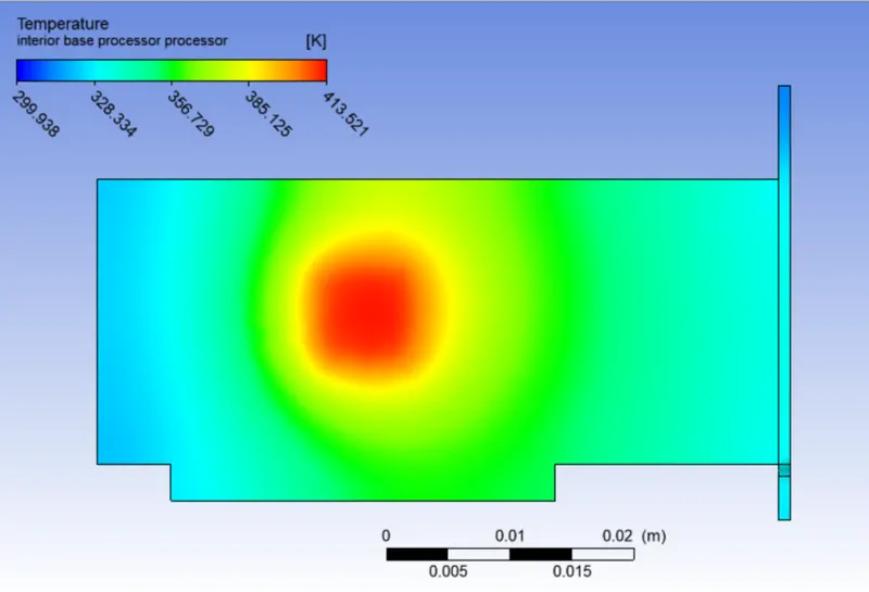
- Find out the maximum temperature and heat transfer coefficient attained by the processor.
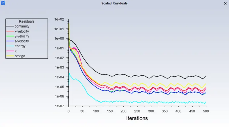
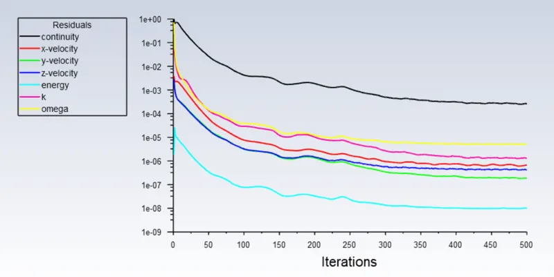
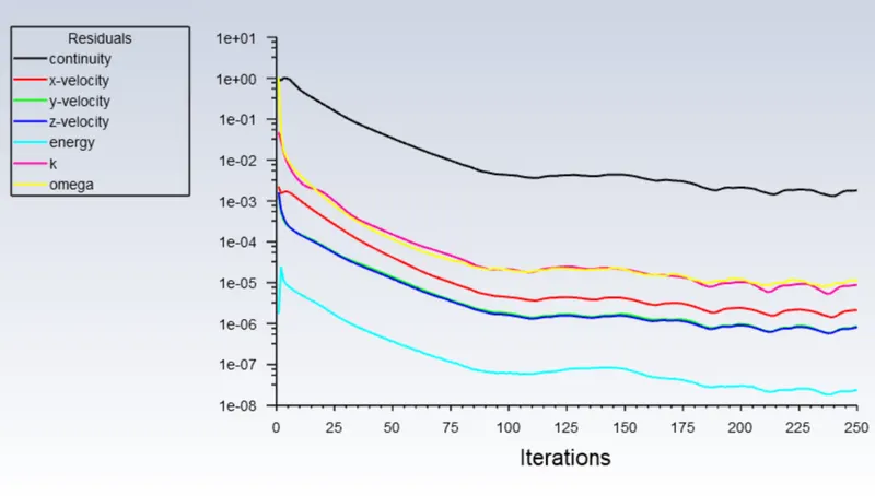
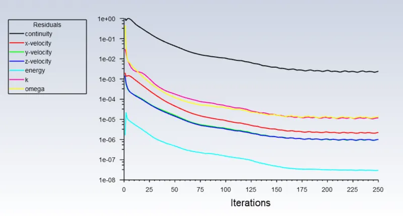
- Prove that the simulation has achieved convergence with appropriate images and plots.
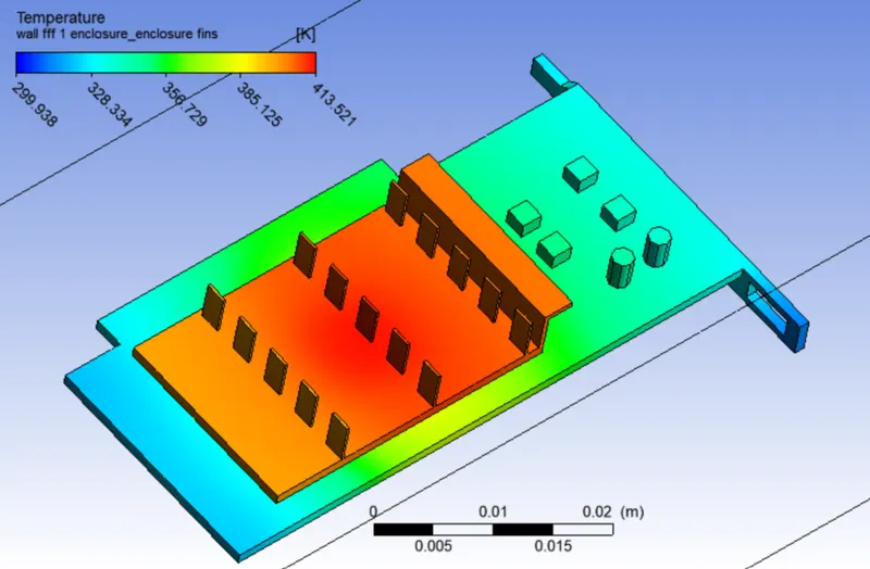
- Identify potential hotspots on the model.
THEORY –
Conjugate Heat Transfer (CHT) - Conjugate heat transfer corresponds with the combination of heat transfer in solids and heat transfer in fluids. In solids, conduction often dominates whereas in fluids, convection usually dominates. In simple words, it is the heat transfer between solid and fluid simultaneously. There is a thermal coupling at the interfaces of two regions. Conjugate heat transfer is observed in many situations. For example, heat sinks are optimized to combine heat transfer by conduction in the heat sink with the convection in the surrounding fluid.
As the technology is evolving, the need for better, faster and more efficient GRAPHIC CARD is also increasing. Graphic card is one of the most essential components of any product and hence it performing operations almost all the time and in order to ensure that the performance of graphic card is not dropping due to the heat produced by the graphic card, the dissipation of this heat is one of the most essential tasks. If the heat is not getting dissipated, over a larger period of time the graphic card will get damaged and its performance will decrease drastically and hence it’s important to do The Conjugate Heat Transfer (CHT) analysis on a graphic card and in this paper that’s what we’ll be analyzing.
CHT Analysis on a Graphics card -
Geometry -
- Load the Graphic card model in the Spaceclaim.
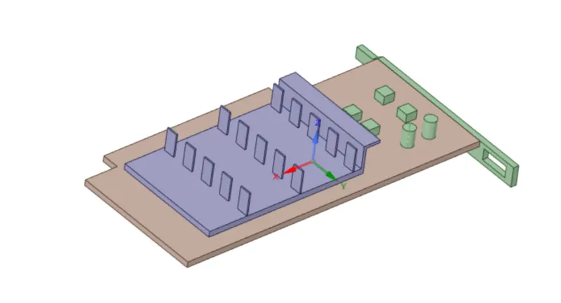
- Divide the model into proper components such as fins, processor, base etc.
- Enclosure is already given with the geometry.
- This completes our geometry.
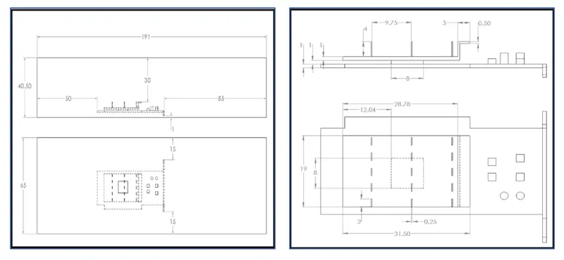
Dimensions of the Model -
Model -
CASE 1 - BASE LINE MESH WITH INLET VELOCITY OF 1m/s
Mesh -
- Start the mesh section
- Name each component such as base, fin, processor etc.
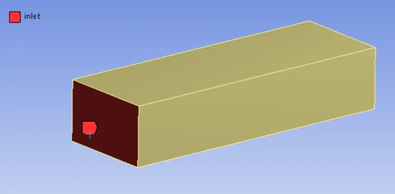
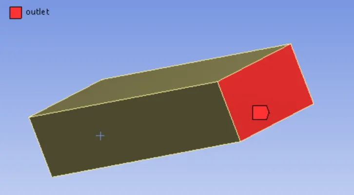
- Name the boundaries such as inlet, outlet and wall.
- Generate the mesh and then edit it with mesh size
Generated Mesh -
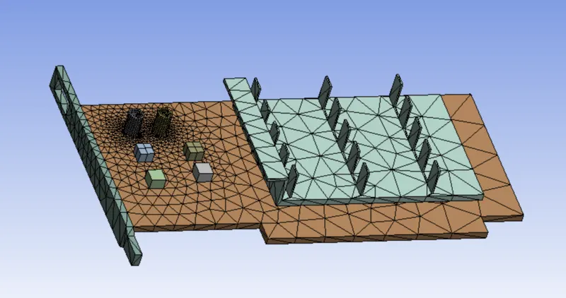
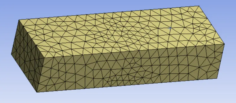
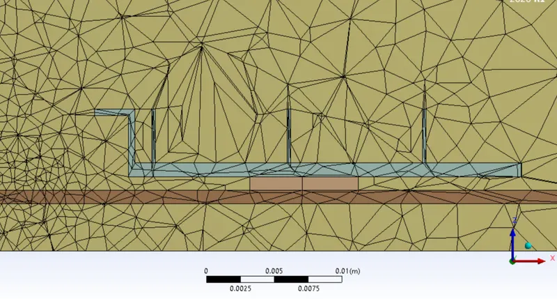
As we move from one component to another, we can clearly see that the mesh is connected perfectly between the components and hence our mesh is conformal mesh which was required.
Named Selections -
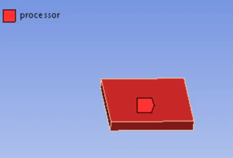
Processor -
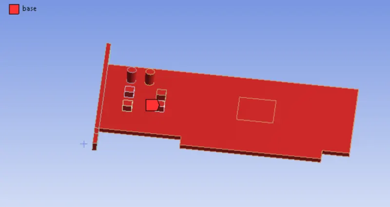
Base -
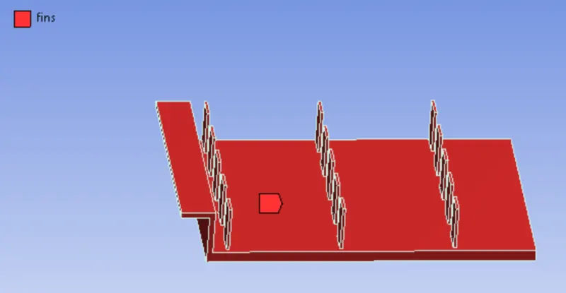
Fins -
Inlet -
Outlet -
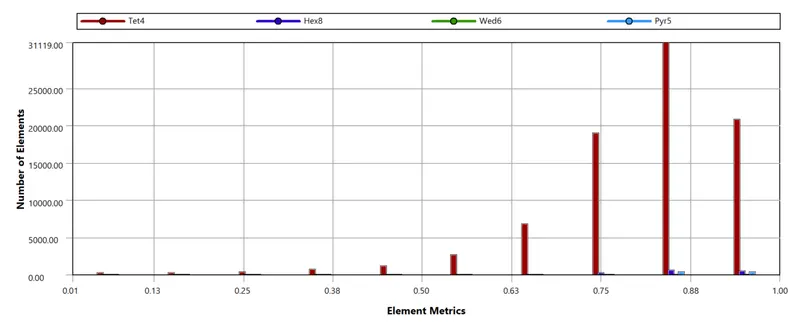
In order to see if the mesh we have generated is accurate or not, we'll check a quantity known as orthogonal mesh quality which tells us about the quality of our mesh.
Element Quality -
SETUP -
Setting up the physics for CHT analysis on a graphics card in ANSYS fluent.
- For this case we are using pressure-based steady state solver
- Velocity formulation - Absolute
Model setup
- Energy
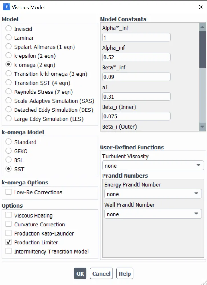
- Viscous - k-omega (SST)
Materials -
For Fluid: Air
- Density - `1.225 (kg)/m^3`
- Viscosity - `1.7894 e^-5 (kg)/(ms)`
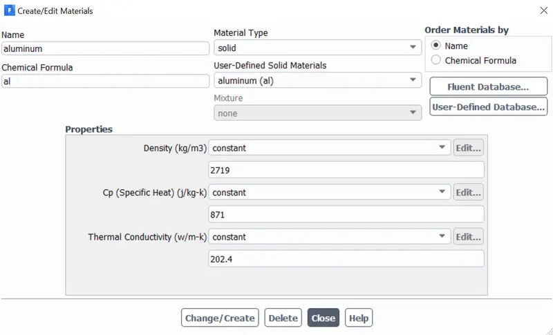
For Fins: Aluminum
- Density - `2719 (kg)/m^3`
- Specific Heat - `871(J)/(kg*K)`
- Thermal Conductivity - `202.4 W/(m*K)`
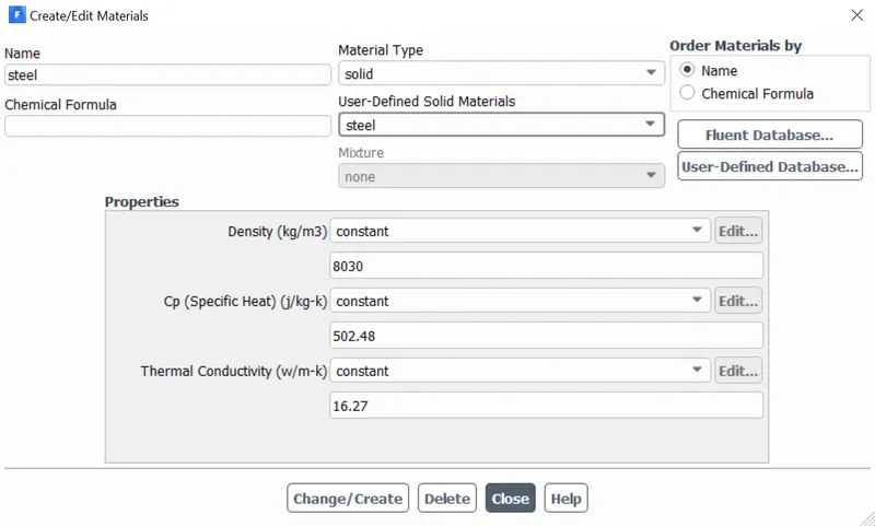
For Base: Steel
- Density - `8030(kg)/m^3`
- Specific Heat - `502.48(J)/(kg*K)`
- Thermal Conductivity - `16.27W/(m*K)`
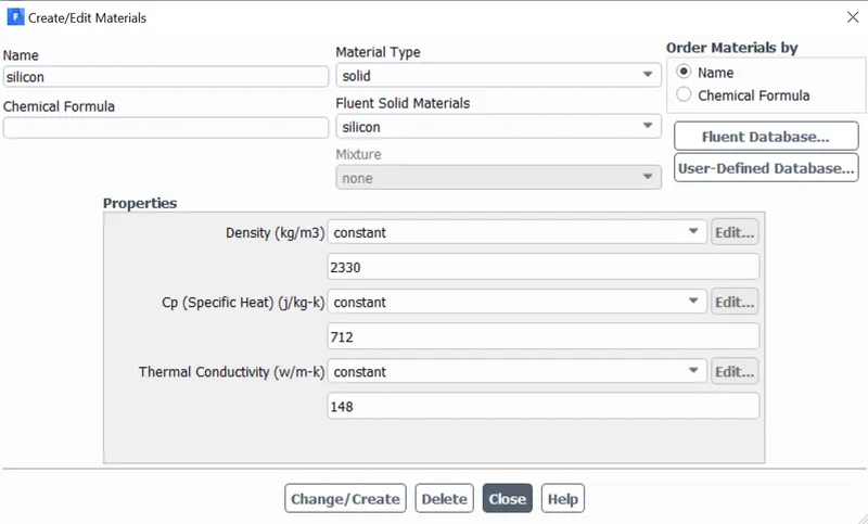
For Processor: Silicon
- Density - `2330(kg)/m^3`
- Specific Heat - `712(J)/(kg*K)`
- Thermal Conductivity - `148W/(m*K)`
Setting up the source terms:
For this case we consider that, our processor is a source terms and it generating heat.
So, for setting up the source term go to Zones - Cell zones - and dick on the processor for editing which is in the Solid.
After that select the material to gold and dick on the source terms to enabled it and set the energy source to 1.
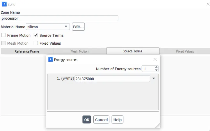
Calculation for the Energy source:
Let the processor consumed by the processor (P) = 15W.
Volume of the processor (V) = 8*8*1 mm^3
So, Energy produced by the processor = P/V = 234375000 W/m^3.
Boundary Conditions -
Inlet
- Air is used as a inlet fluid
- Velocity =1 m/s
- Temperature = 300 K
Outlet
- Pressure = Gauge pressure (0 pa)
Since we're done with setting up everything, now we can run our simulation and see the results.
Results -
Residuals -
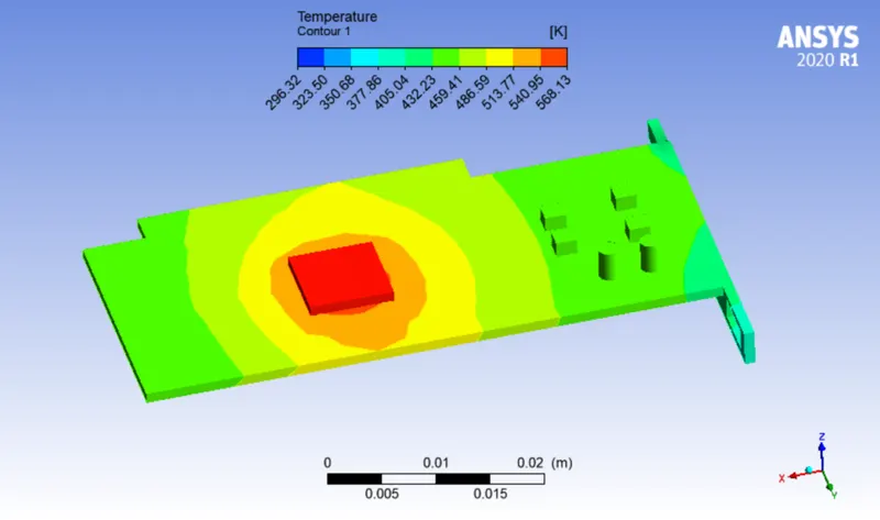
Temperature Distribution of different components -
Processor and Base -
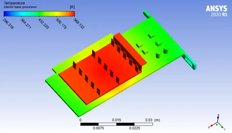
Fins -
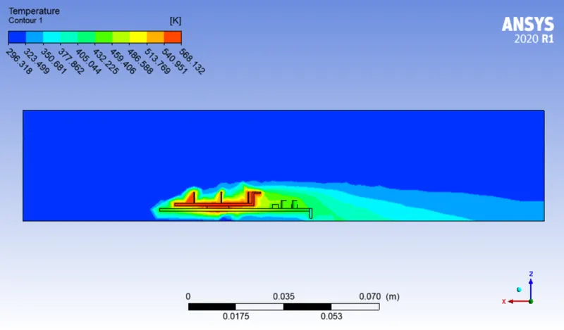
Global Temperature Contour -
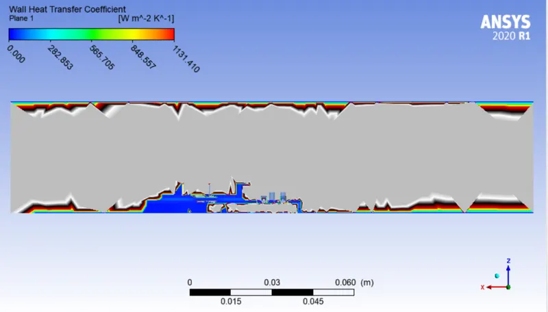
Wall Heat Transfer Coefficient -
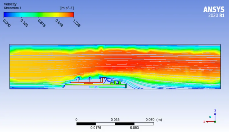
Velocity Streamline plot -
CASE 2 - REFFINED MESH WITH DIFFERENT INLET VELOCITY
Mesh -
We'll refine our base line mesh for this simulation.
Global mesh setting of element size = 2 mm
1) PCB body sizing element size =1 mm
2) Proc body sizing element size = 0.5 mm
3) Fins body sizing element size = 0.5 mm
Number of elements = 3,86,570
Generated Mesh -
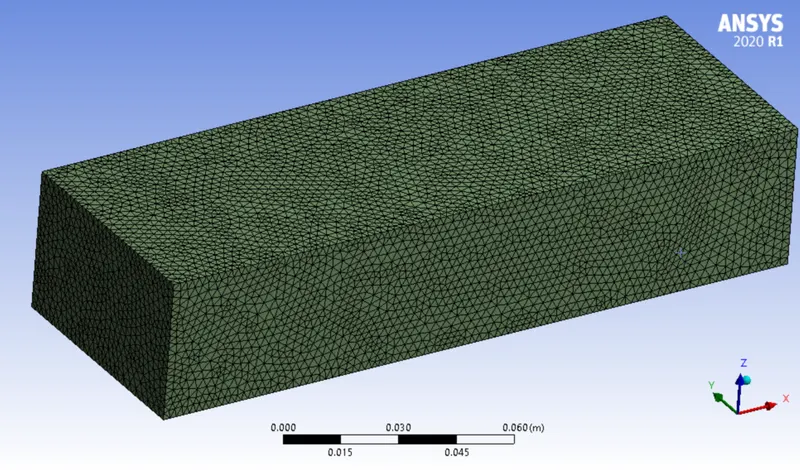
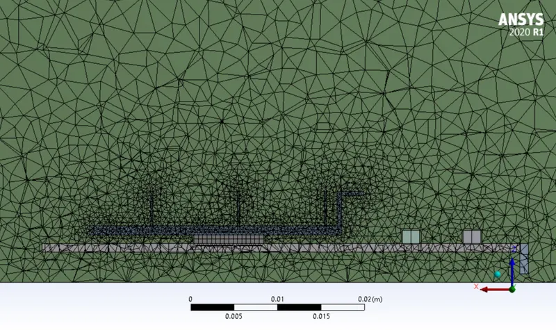
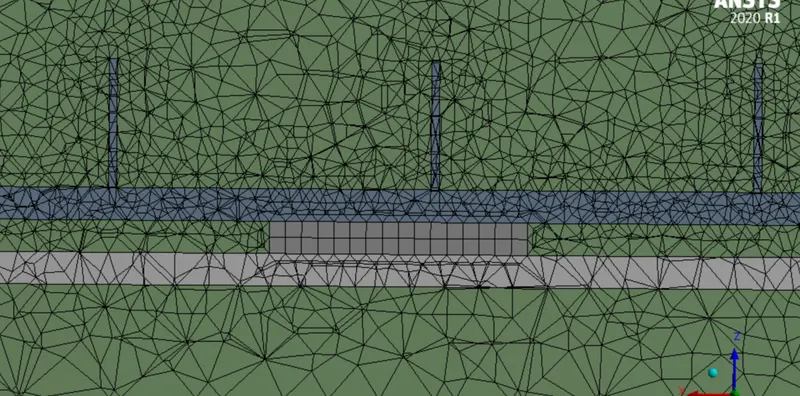
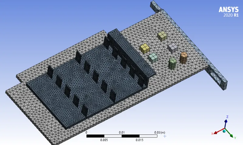
As we move from one component to another, we can clearly see that the mesh is connected perfectly between the components and hence our mesh is conformal mesh which was required.
In order to see if the mesh we have generated is accurate or not, we'll check a quantity known as orthogonal mesh quality which tells us about the quality of our mesh.
Element Quality -
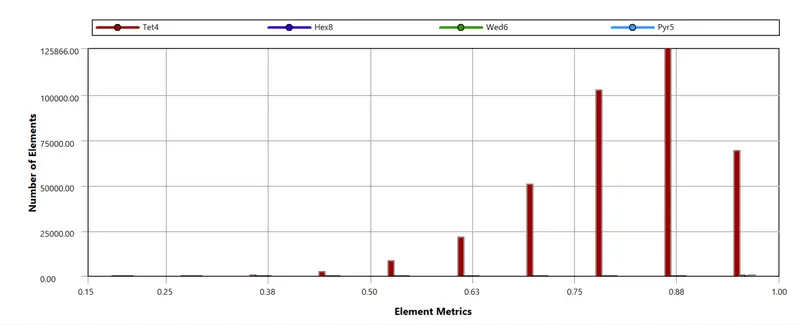
PART A - Inlet Velocity = 3 m/s
SETUP -
Setup is same as in the case 1 with inlet velocity = 5m/s.
Results -
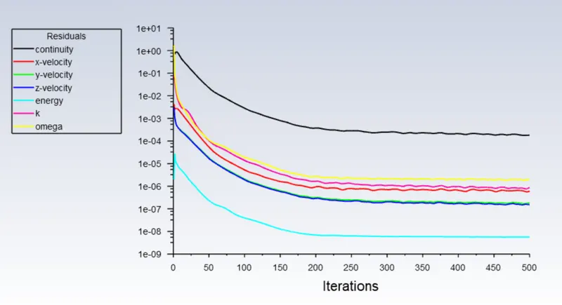
Residuals -
Temperature Distribution of different components -
Processor and Base -
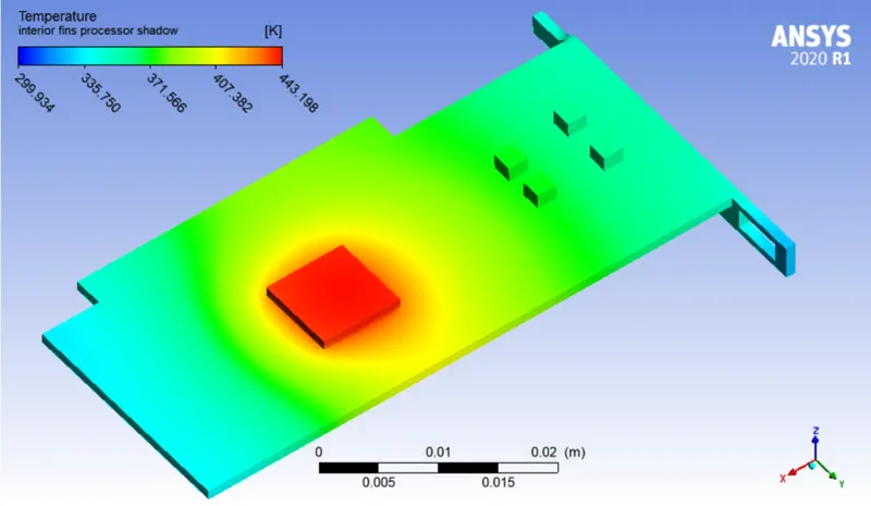
Fins -
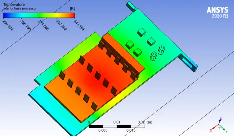
Global Temperature Contour -
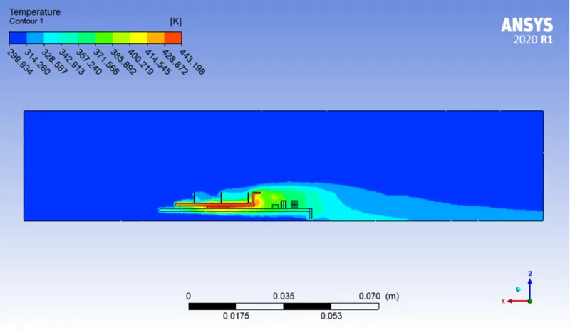
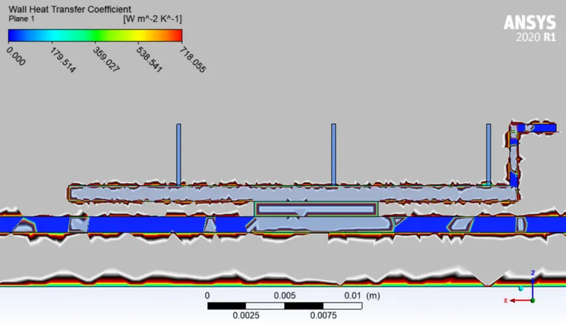
Wall Heat Transfer Coefficient -
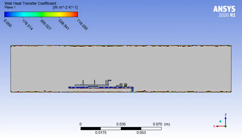
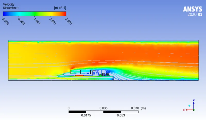
Velocity Streamline plot -
PART B - Inlet Velocity = 5 m/s
SETUP -
Setup is same as in the case 1 with inlet velocity = 5m/s.
Results -
Residuals -
Temperature Distribution of different components -
Processor and Base -
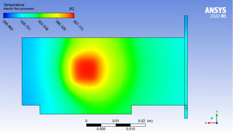
Fins -
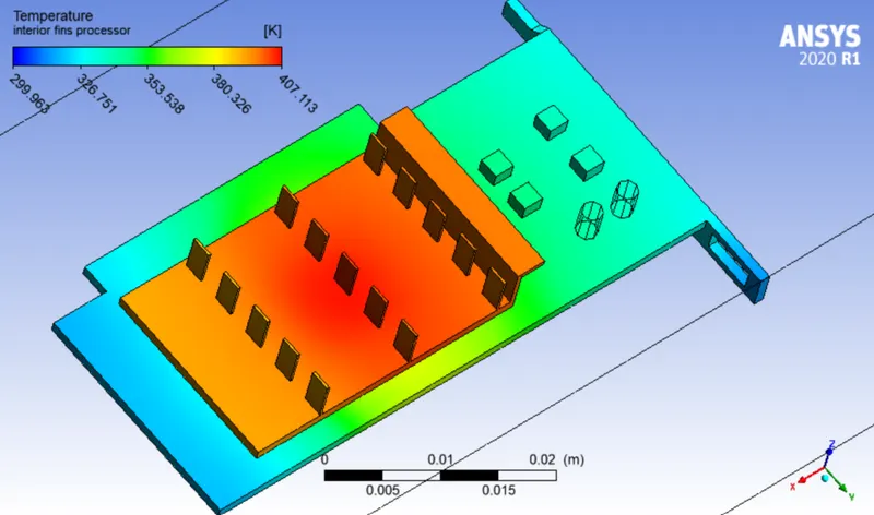
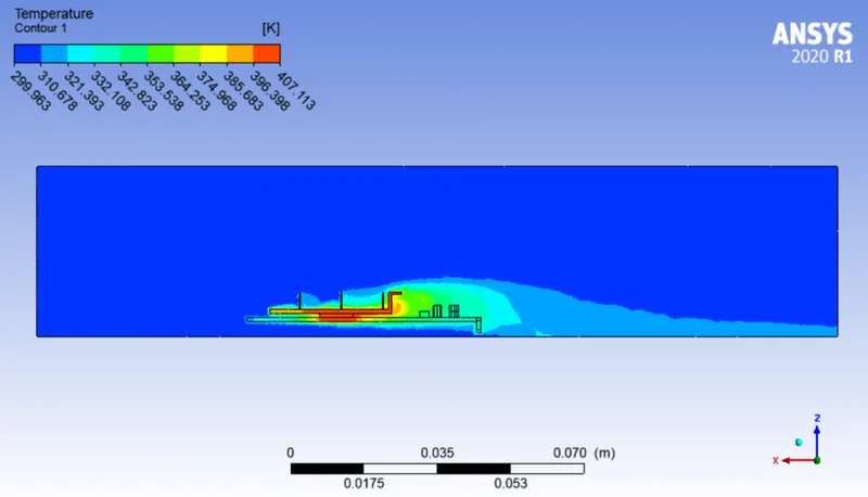
Global Temperature Contour -
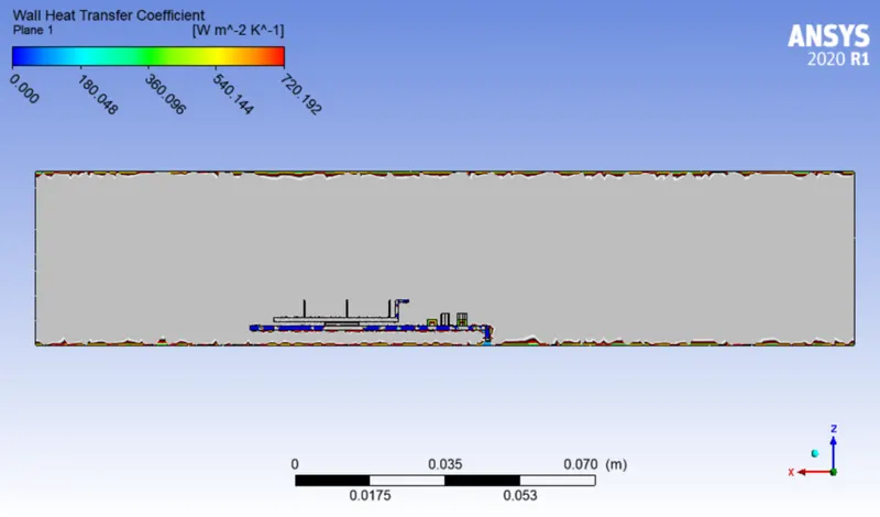
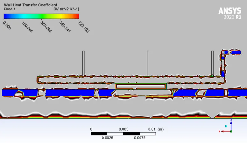
Wall Heat Transfer Coefficient -
Velocity Streamline plot -
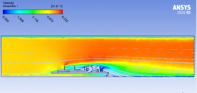
CASE 3 - ADDING A SECOND ENCLOSURE FOR DIFFERENT INLET VELOCITY
Geometry -
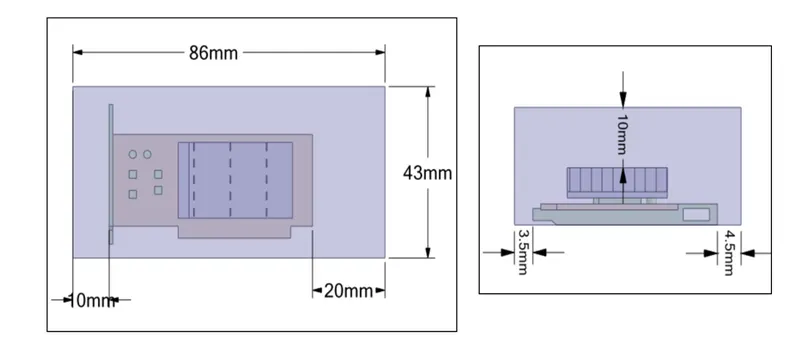
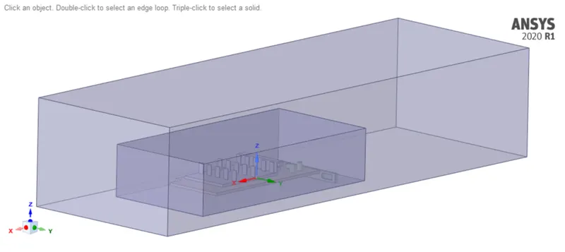
In order to refine the mesh and keep the element numbers to a minimum, an enclosure is made surrounding the graphics card. An important step while doing this is selecting all three bodies (fins, processor, PCB) and then applying enclosure feature in ANSYS Fluent. The outer enclosure is deleted and then created again by selecting inner enclosure. The image below gives information of dimensions needed to make the enclosures.
Mesh -
- Body sizing - Outer Enclosure
Element size = 2 mm
Behavior - Hard - Body sizing - Inner Enclosure
Element size = 1 mm
Behavior - Hard - Body sizing = Base
Element size = 1 mm
Behavior - Hard - Body sizing - Processor
Element size = 0.5 mm
Behavior - Hard - Body sizing - Fin
Element size = 0.5 mm
Behavior - Hard
Number of elements = 11,61,388
Generated Mesh -
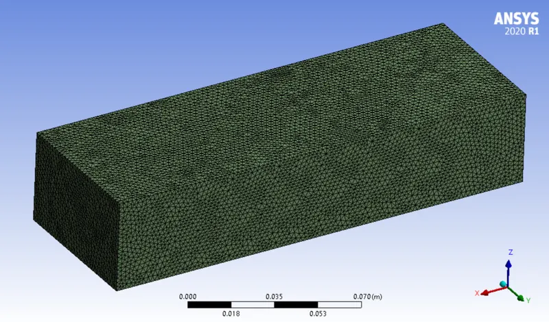
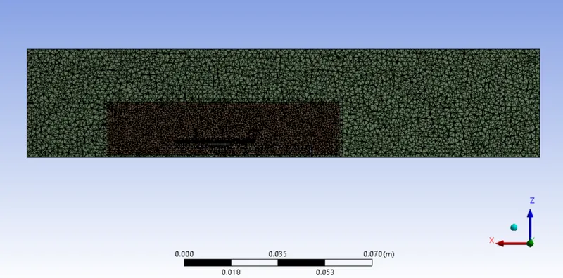
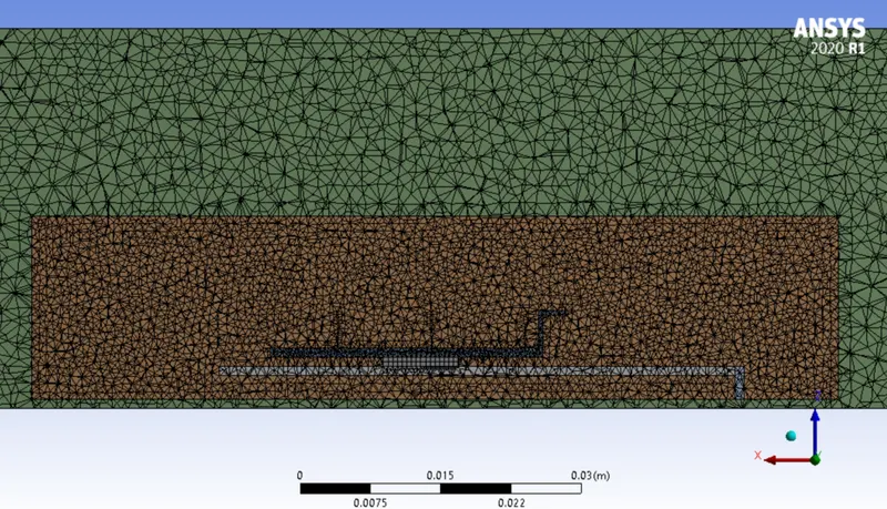
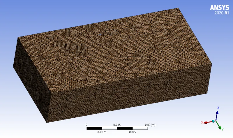
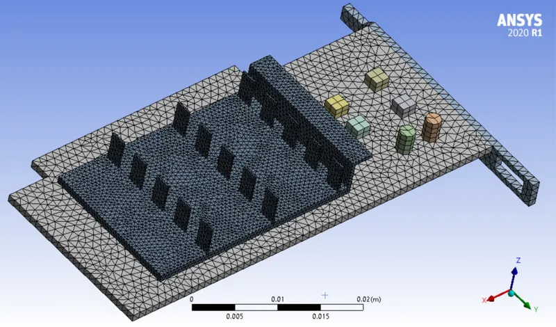
As we move from one component to another, we can clearly see that the mesh is connected perfectly between the components and hence our mesh is conformal mesh which was required.
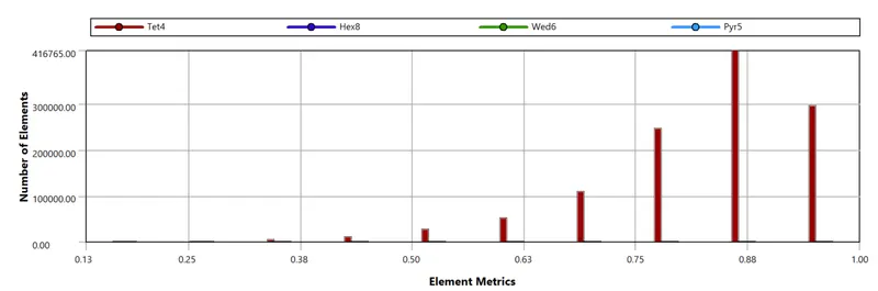
In order to see if the mesh we have generated is accurate or not, we'll check a quantity known as orthogonal mesh quality which tells us about the quality of our mesh.
Element Quality -
PART A - Inlet Velocity = 1 m/s
SETUP -
Setup is same as in the above cases with inlet velocity = 1m/s.
Results -
Residuals -
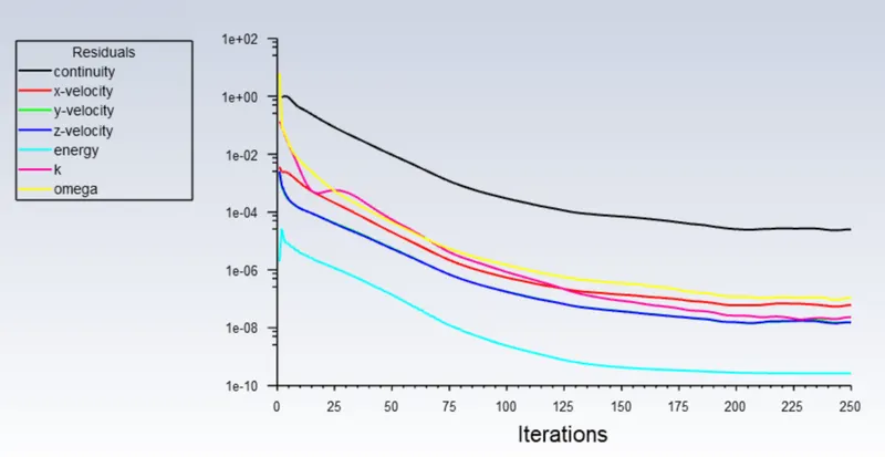
Temperature Distribution of different components -
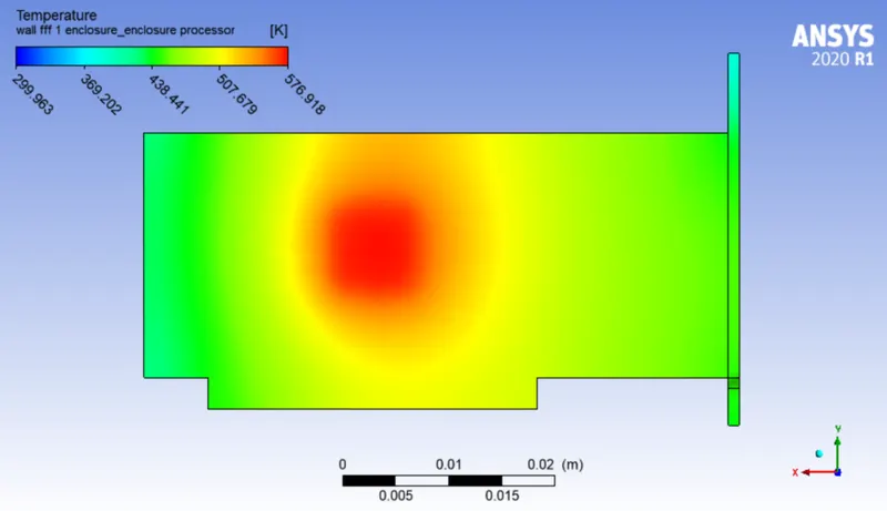
Processor and Base -
Fins -
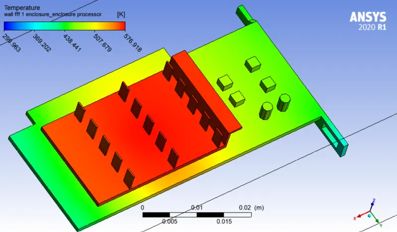
Global Temperature Contour -
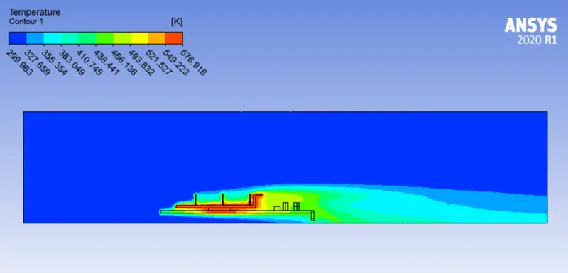
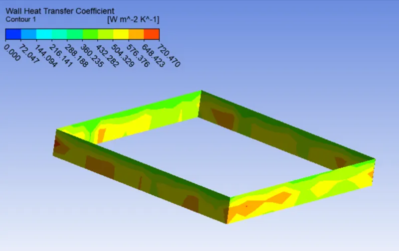
Wall Heat Transfer Coefficient -
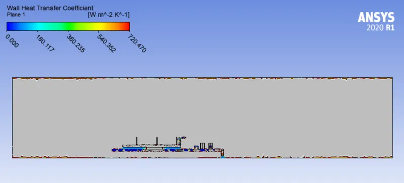
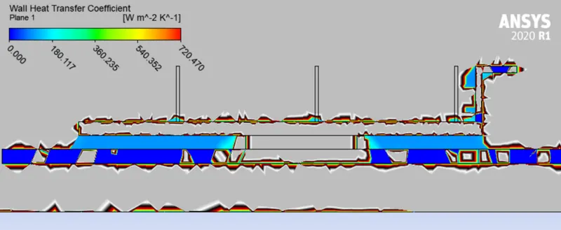
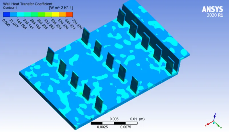
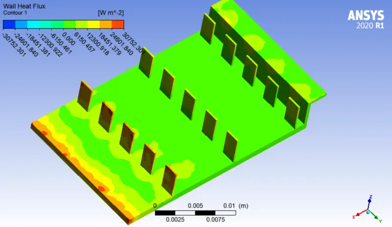
Wall Heat Flux -
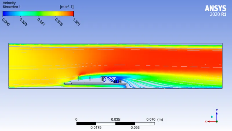
Velocity Streamline plot -
PART B - Inlet Velocity = 3 m/s
SETUP -
Setup is same as in the above cases with inlet velocity = 3m/s.
Results -
Residuals -
Temperature Distribution of different components -
Processor and Base -
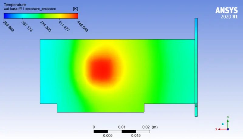
Fins -
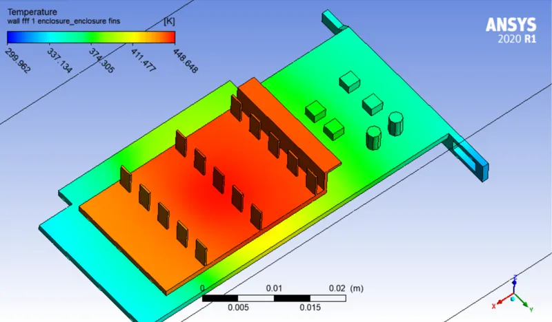
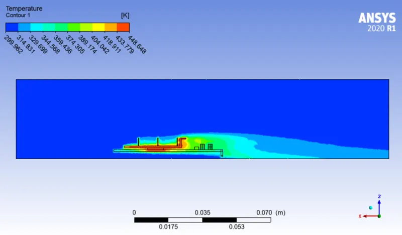
Global Temperature Contour -
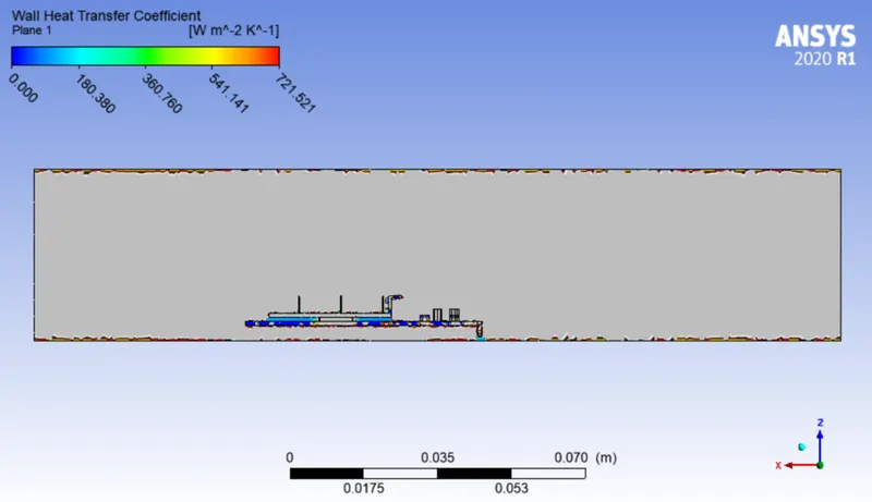
Wall Heat Transfer Coefficient -
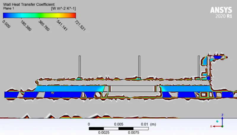
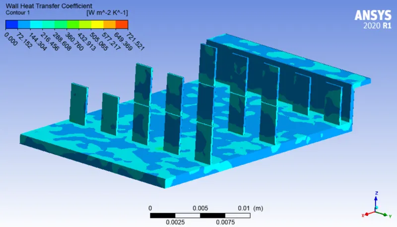
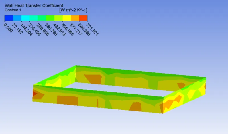
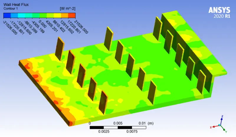
Wall Heat Flux -
Velocity Streamline plot -
PART C - Inlet Velocity = 5m/s
SETUP -
Setup is same as in the above cases with inlet velocity = 5m/s.
Results -
Residuals -
Temperature Distribution of different components -
Processor and Base -
Fins -
Global Temperature Contour -
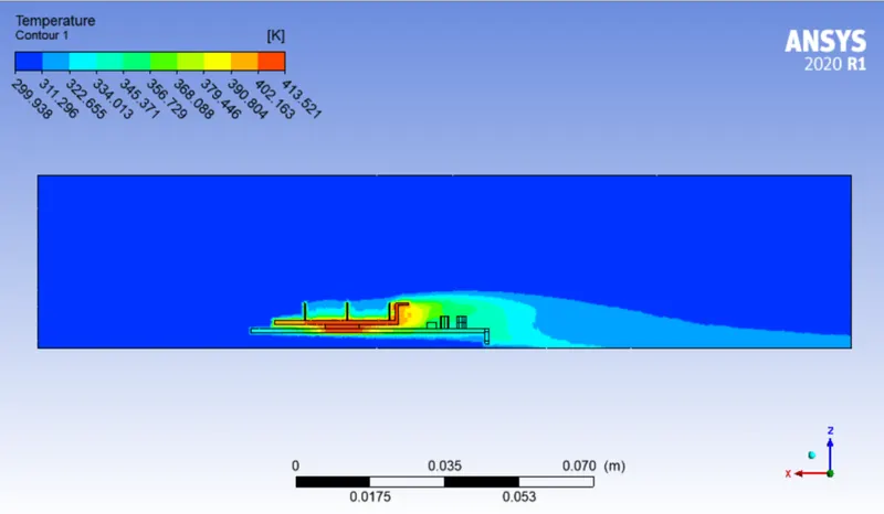
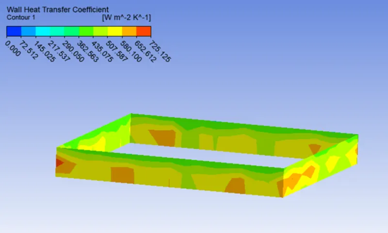
Wall Heat Transfer Coefficient -
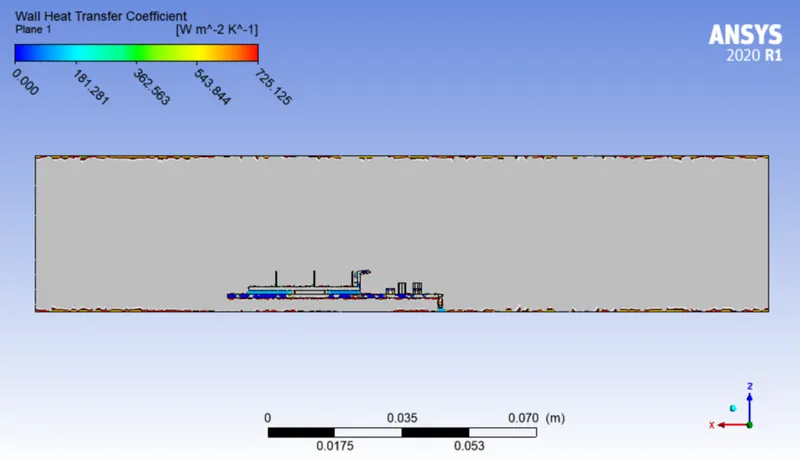
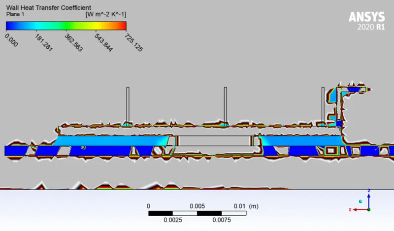
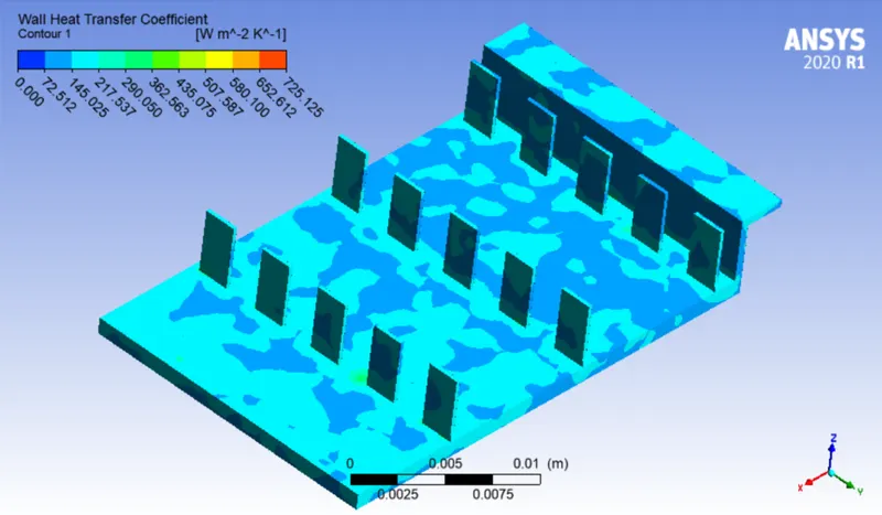
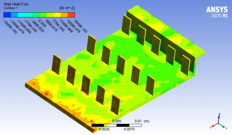
Wall Heat Flux -
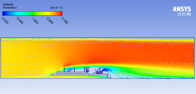
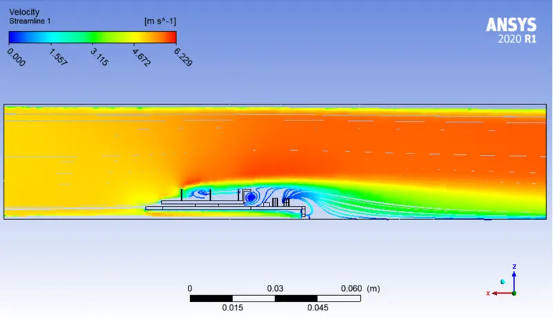
Velocity Steamline plot -
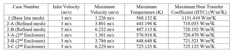
Comparison -
We can look at the comparison between different mesh and also between different velocities in the table given below.
Conclusion -
- If we look at the heat flux distribution at the fins, we can see that the heat flux seems to be more from front end. This is due to higher temperature difference in solid and fluid. As the air moves forward, it takes less heat, so the region appears green.
- The heat flux distribution over a fin is as expected. As the corners and centers have a higher contact with air, so they give up more heat.
- While if we look at the temperature distribution at the fin, it can be seen that fins at the front are cooler than the ones behind. This happens because the cold air first hits the front fins, it gets heated up and goes to next fin. Hence, the next fins can't give it enough heat as difference in temperature is lower in between solid and fluid. In Simple terms, the fins at the front release more heat, as seen through the heat flux distribution, as compared to the fins at the back and hence the fins at the front are getting cooler/releasing heat faster than the fins at the back.
- A potential hotspot is also present below processor, on the areas around the processor on the base. So, one must avoid placing components on that place.
- For the turbulent models, we have to take care of the assumptions and the boundary conditions we use as the accuracy of our simulation depends on it.
- As we’re doing a CHT analysis, we need to make sure to use a model that gives accurate heat transfer near wall meaning a model which can handle the near wall analysis. And hence we’re using the K-w (SST) model, because this model is useful when we need near wall analysis.
- Mesh/ grid dependency test is very important to get confidence over results.