Week 7 - Simulation of a 1D Super-sonic nozzle flow simulation using Macormack Method
OBJECTIVE – Simulation of 1D Super-sonic nozzle flow simulation using Macormack method.
THEORY – In this study we’re going to simulate flow inside a convergent-divergent nozzle as shown below. The inlet of the nozzle is connected to a reservoir, the cross section of the reservoir is very large and hence the inlet velocity of the flow is very low. The flow is sub sonic in convergent section and it becomes supersonic as it flows through divergent section.
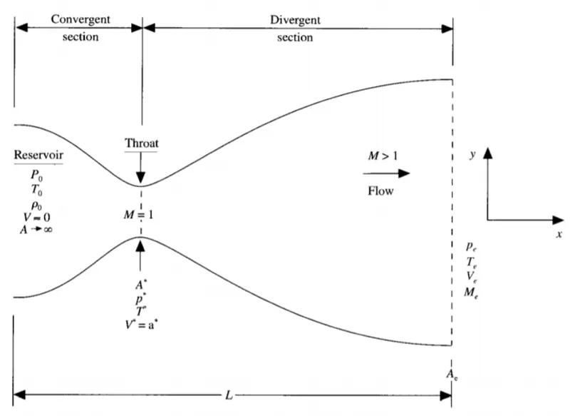
GOVERNING EQUATIONS –
To get the governing equations, let’s consider a small control volume/area as shown below.
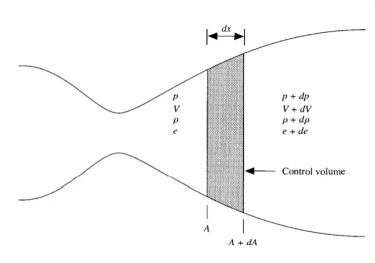
The length of the control volume is dx and since dx is very small, the flow variables does not change along the small control volume and hence are uniform. Although in reality the flow variables change in both the direction. But we’re only considering 1D flow and hence this flow is known as quasi 1D flow.
The governing equations can be expressed in conservative or non-conservative form for continuity, momentum and energy equation in terms of non-dimensionalized variables.
NON - CONSERVATIVE FORM -
Non – Conservative Continuity Equation -
`(∂ρ^')/(∂t^' )=-ρ^' ((∂V^')/(∂x^' ))-ρ^' V^' (∂(lnA^' )/(∂x^' ))-V^' ((∂ρ^')/(∂x^' ))`
Non – Conservative Momentum Equation -
`(∂V^')/(∂t^' )=-V^' ((∂V^')/(∂x^' ))-(1/γ)((∂T^')/(∂x^' )+T^'/ρ^' ((∂ρ^')/(∂x^' )))`
Non – Conservative Energy Equation -
`(∂T^')/(∂t^' )=-V^' ((∂T^')/(∂x^' ))-(γ-1)T^' [(∂V^')/(∂x^' )+V^' ∂(lnA^' )/(∂x^' )]`
To solve the above given equation, we can either follow the method we have used before that is using the first order approximation to find the derivatives and then using time marching to solve the equations, but in this study to get a better result we’ll use a method known as macormack method.
In this method we can get second order approximation for derivative without using the long and lengthy formula for second order approximation and hence this method is very useful.
MACORMACK METHOD -
Let f(x) be the equation to be solved, the following steps are done to solve the equation using the macormack method.
1.) Initial guess -
Before solving the equation, we need to make an initial guess for all the variables like density, temperature and velocity.
2.) Predector Step -
In this step we solve the given equation using the forward difference method and the initial guess.
`((df)/(dt))_p=(f(i+1)-f(i))/(Δx)`
3.) Initial value update -
In this step we'll update our initial guess values using the values we get from the predector step.
`f_p=f_"Initial " +((df)/(dt))_p⋅Δt`
f_p = value from the predector step
4.) Corrector step -
In this step we solve the given equation using the backward difference method and the new updated values we get from step three.
`((df)/(dt))_p=(f(i)-f(i-1))/(Δx)`
5.) Average value -
As we now have derivative from both forward difference method (2nd step) and the backward difference method (4th step), we can use these values to get an average value that will be 2nd order approximate and hence will impove our result.
`((df)/(dt))_(avg) = 0.5(((df)/(dt))_p + ((df)/(dt))_c )`
6.) Finale solution update -
Now using the 2nd order approximation derivate we get in 5th step; we can now update our initial guess to a more precise and better approximation and hence we can have faster convergence.
`f_(sol) = f_"Initial " +((df)/(dt))_"avg"⋅Δt`
We'll use all the above step for each time step in order to keep updating our values to get faster convergence and better accuracy.
Initial and Boundary Conditions for Non-Conservative form -
Initial Conditions -
A = 1 + 2.2(x - 1.5)^2 0 <= x <= 3
ρ = 1 - 0.3146*x
T = 1 - 0.2314*x
V = (0.1 + 1.09*x)*(T^(1/2))
Boundary Conditions -
At grid point 1
`ρ_1 = 1`
`T_1 = 1`
`V_1 = 2V_2 - V_3`
At grid point n
`V_n = 2V_(n-1) - V_(n-2)`
`T_n = 2T_(n-1) - T_(n-2)`
`ρ_n = 2ρ_(n-1) - ρ_(n-2)`
CONSERVATIVE FORM -
Conservative Continutiy Equation -
`(∂(ρ^' A^' ))/(∂t^' )+(∂(ρ^' A^' V^' ))/(∂x^' )=0`
Conservative Momentum Equation -
`(∂(ρ^' A^' V^' ))/(∂t^' )+(∂[ρ^' A^' (V^' )^2+(1/γ) ρ^' A^' ])/(∂x^' )=(1/γ) ρ^' ((∂A^')/(∂x^' ))`
Conservative Energy Equation -
`(∂[ρ^' (e^'/(γ-1)+(γ/2) (V^' )^2 ) A^' ])/(∂t^' )+(∂[ρ^' (e^'/(γ-1)+(γ/2) (V^' )^2 ) V^' A^'+ρ^' A^' V^' ])/(∂x^' )=0`
To solve the conservative form equations, we'll have to first convert these equations into the generic form of the governing equations for unsteady, three-dimensional flow.
The equations for quasi one-dimensional flow can be expressed in a similar generic form. Let us define the elements of the solutions vector U, the flux vector F, and the source term J as follows.
`U_1 =ρ^' A^'`
`U_2=ρ^' A^' V^'`
`U_3=ρ^' (e^'/(γ-1)+γ/2 (V^2)' ) A^'`
`F_1 = ρ^' A^' V^'`
`F_2 =ρ^' A^' V^'2+1/γ p^' A^'`
`F_3 =ρ^' (e^'/(γ-1)+γ/2 V^'2 ) V^' A^'+p^' A^' V^'`
`J_2 = 1/γ p^' (∂A^')/(∂x^' )`
With these elements we can write the governing equation for the conservative form as -
`(∂U_1)/(∂t^' )=-(∂F_1)/(∂x^' )`
`(∂U_2)/(∂t^' )=-(∂F_2)/(∂x^' )+J_2`
`(∂U_3)/(∂t^' )=-(∂F_3)/(∂x^' )`
To obtain the primitive variables (p, V, T, etc.), we must decode the elements U1, U2, and U3 as follows. From the definitions of U_1 , U_2 , and U_3 given above, we have
`ρ^' =U_1/A^'`
`V^' =U_2/U_1`
`T^' =e^'=(γ-1)(U_3/U_1 -γ/2 V^'2 )`
`p^'=ρ^' T^'`
As we can see that the flux terms are dependent on primitive variables and not on the solution vector, it’s better to expresses them in terms of solution vectors to avoid the occurrence of instabilities in the final solution. The flux vector in terms of solution vector is given as -
`F_1 = U_2`
`F_2=(U_2^2)/U_1 +(γ-1)/γ (U_3-γ/2 (U_2^2)/U_1 )`
`F_3=γ (U_2 U_3)/U_1 -(γ(γ-1))/2 (U_2^3)/(U_1^2 )`
Initial and Boundary Conditions for Conservative form -
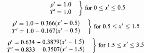
Initial Conditions -
A = 1 + 2.2(x - 1.5)^2 0 <= x <= 3
Boundary Conditions -
At grid point 1
`U_(1(i=1))=ρ^' (1)⋅A^' (1)`
`U_(2(i=1))=2U_(2(i=2))-U_(2(i=3))`
`U_(3(i=1))=U_1 (T^'/(γ-1)+γ/2 V^'2 )`
At grid point n
`U_(1(i=n))=2U_(1(i=n-1))-U_(1(i=n-2))`
`U_(2(i=n))=2U_(2(i=n-1))-U_(2(i=n-2))`
`U_(3(i=n))=2U_(3(i=n-1))-U_(3(i=n-2))`
Now since we're done with defining the governing equation for both conservative and non-conservative form as well as their initial and boundary conditions, we can now write a MATLAB code to solve these equations.
MAIN MATLAB CODE -
clear all
close all
clc

% Inputs
l = 3;  % Length of the nozzel
n = [31,61,91]; % Number of grid points
c = 0.5; % CFL number

% Time step
nt = 1400;

for i = 1:length(n)

    % Grid points
    x = linspace(0,l,n(i));

    % Area
    a = 1 + 2.2*(x - 1.5).^2 ; % Area of the nozzel at different grid points
    throat = find( a == 1);    % Finding the grid point for throat

    [v_nc,T_nc,rho_nc,mfr_nc,mfr_throat_nc] = non_conservation_form (n(i),l,nt,c,a,throat) ;
    [rho_c,T_c,v_c,mfr_c,mfr_throat_c] = conservation_form(n(i),l,nt,c,a,throat) ;

    h = linspace(0,nt,nt);

    if n(i) == 31
        figure(7)
        subplot(2,1,1)
        plot(h,mfr_throat_nc,'b',h,mfr_throat_c,'r')
        legend('Non-Conservative form','Conservative form')
        xlabel('Time Step (nt)')
        ylabel('Mass flow rate')
        title('Mass flow rate for "Non-Conservative form vs Conservative form" at throat')

        subplot(2,1,2)
        plot(x,mfr_nc,'b',x,mfr_c,'r')
        xlabel('Length of the nozzel')
        ylabel('Mass flow rate')
        title('Mass flow rate for "Non-Conservative form vs Conservative form" along the nozzel')
    end

    figure(8)
    subplot(2,1,1)
    plot(h,mfr_throat_nc)
    hold on
    xlabel('Time Step (nt)')
    ylabel('Mass flow rate')
    legend('@31 nodes','@61 nodes','@91 nodes')
    title('Non-Conservative form : Grid independency test at throat')

    subplot(2,1,2)
    plot(h,mfr_throat_c)
    hold on
    xlabel('Time Step (nt)')
    ylabel('Mass flow rate')
    title('Conservative form : Grid independency test at throat')

    figure(9)
    subplot(2,1,1)
    plot(x,mfr_nc)
    hold on
    xlabel('Time Step (nt)')
    ylabel('Mass flow rate')
    legend('@31 nodes','@61 nodes','@91 nodes')
    title('Non-Conservative form : Grid independency test along the nozzel')

    subplot(2,1,2)
    plot(x,mfr_c)
    hold on
    xlabel('Time Step (nt)')
    ylabel('Mass flow rate')
    title('Conservative form : Grid independency test along the nozzel')

end
We've used two functions in the above code, one for conservative form and one for non-conservative form, which are shown below.
NON-CONSERVATIVE FORM FUNCTION -
function [v,T,rho,mass_flow_rate,mfr_throat] = non_conservation_form (n,l,nt,c,a,throat)

% Grid
x = linspace(0,l,n);
dx = x(2) - x(1);

% Initial conditions
rho = 1 - 0.3146*x ;
T = 1 - 0.2314*x ;
v = (0.1 + 0.9*x).*(T.^0.5);
gamma = 1.4;

for k = 1:nt
    dt = min((c*dx)./(sqrt(T) + v));

    rho_old = rho ;
    v_old = v;
    T_old = T;

    % Predictor step

    for j = 2:n-1

        dv_dx = (v(j+1) - v(j))/dx ;
        drho_dx = (rho(j+1) - rho(j))/dx ;
        dT_dx = (T(j+1) - T(j))/dx ;
        dlogA_dx = (log(a(j+1)) - log(a(j)))/dx ;

        % Continutiy equation
        drho_dt_p(j) = -rho(j)*dv_dx - rho(j)*v(j)*dlogA_dx - v(j)*drho_dx ;

        % Momentum equation
        dv_dt_p(j) = -v(j)*dv_dx - (1/gamma)*(dT_dx + (T(j)/rho(j))*drho_dx) ;

        % Energy equation
        dT_dt_p(j) = -v(j)*dT_dx - (gamma - 1)*T(j)*(dv_dx + v(j)*dlogA_dx) ;

        % Solution update
        rho(j) = rho(j) + drho_dt_p(j)*dt ;
        v(j) = v(j) + dv_dt_p(j)*dt ;
        T(j) = T(j) + dT_dt_p(j)*dt ;
    end

    % Corrector step

    for j = 2:n-1

        dv_dx = (v(j) - v(j-1))/dx ;
        drho_dx = (rho(j) - rho(j-1))/dx ;
        dT_dx = (T(j) - T(j-1))/dx ;
        dlogA_dx = (log(a(j)) - log(a(j-1)))/dx ;

        % Continutiy equation
        drho_dt_c(j) = -rho(j)*dv_dx - rho(j)*v(j)*dlogA_dx - v(j)*drho_dx ;

        % Momentum equation
        dv_dt_c(j) = -v(j)*dv_dx - (1/gamma)*(dT_dx + (T(j)/rho(j))*drho_dx) ;

        % Energy equation
        dT_dt_c(j) = -v(j)*dT_dx - (gamma - 1)*T(j)*(dv_dx + v(j)*dlogA_dx) ;

    end

    % Computing the avaerage time derivative

    drho_dt = 0.5*(drho_dt_p + drho_dt_c);
    dv_dt = 0.5*(dv_dt_p + dv_dt_c);
    dT_dt = 0.5*(dT_dt_p + dT_dt_c);

    % Finale solution update

    for i = 2:n-1
        rho(i) = rho_old(i) + drho_dt(i)*dt ;
        v(i) = v_old(i) + dv_dt(i)*dt ;
        T(i) = T_old(i) + dT_dt(i)*dt ;
    end

    % Applying boundary conditions

    % Inlet
    v(1) = 2*v(2) - v(3);

    % Outlet
    v(n) = 2*v(n-1) - v(n-2);
    rho(n) = 2*rho(n-1) - rho(n-2);
    T(n) = 2*T(n-1) - T(n-2);

    % Mass flow rate

    mass_flow_rate = rho.*a.*v ;
    pressure = rho.*T ;
    mach_no = v./(sqrt(T)) ;

    rho_throat(k) = rho(throat);
    v_throat(k) = v(throat);
    T_throat(k) = T(throat);
    pressure_throat(k) = pressure(throat);
    mfr_throat(k) = mass_flow_rate(throat);
    mn_throat(k) = mach_no(throat);

    if n == 31
        figure(1)
        hold on
        if k == 1
            plot(x,mass_flow_rate,'b')
            title('Non-conservation : Variation of mass flow rate distributiin inside the nozzel for 31 nodes')
        elseif k == 51
            plot(x,mass_flow_rate,'g')
        elseif k == 151
            plot(x,mass_flow_rate,'r')
        elseif k == 201
            plot(x,mass_flow_rate,'m')
        elseif k == 700
            plot(x,mass_flow_rate)
        elseif k == 1400
            plot(x,mass_flow_rate)
            xlabel('Length of the nozzel')
            ylabel('Mass flow rate')
            legend('@1','@51','@151','@201','@700','@1400')
        end
    end

end

if n == 31
    figure(2)
    subplot(4,1,1)
    plot(x,v)
    title('Non Conservation : Steady State Distribution Of Primitive Variables for 31 nodes')
    ylabel('Velocity')
    grid on
    subplot(4,1,2)
    plot(x,T)
    ylabel('Temperature')
    grid on
    subplot(4,1,3)
    plot(x,rho)
    ylabel('Density')
    grid on
    subplot(4,1,4)
    plot(x,mach_no)
    ylabel('Mach Number')
    xlabel('Nozzel Length')
    grid on

    h = linspace(0,nt,nt);

    figure(3)
    plot(h,rho_throat);
    title('Non-conservation : Time-wise variation of primitive variable at throat for 31 nodes')
    hold on
    plot(h,v_throat);
    plot(h,T_throat);
    plot(h,pressure_throat);
    plot(h,mfr_throat);
    plot(h,mn_throat);
    legend('Density','Velocity','Temperature','Pressure','Mass flow rate','Mach number')
    xlabel('Time step (nt)')
    ylabel('Primitive variables')
    hold off
end
end
RESULTS FOR NON-CONSERVATIVE FORM -
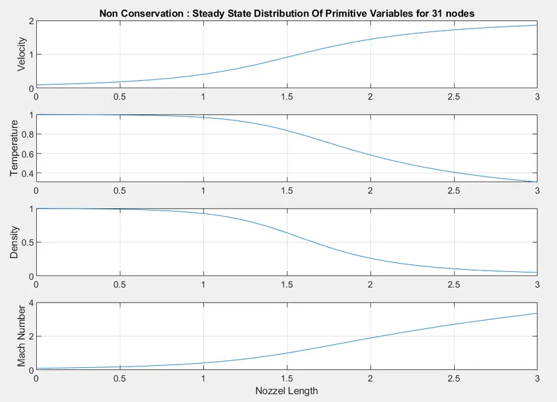
Steady state distribution of primitive variables -
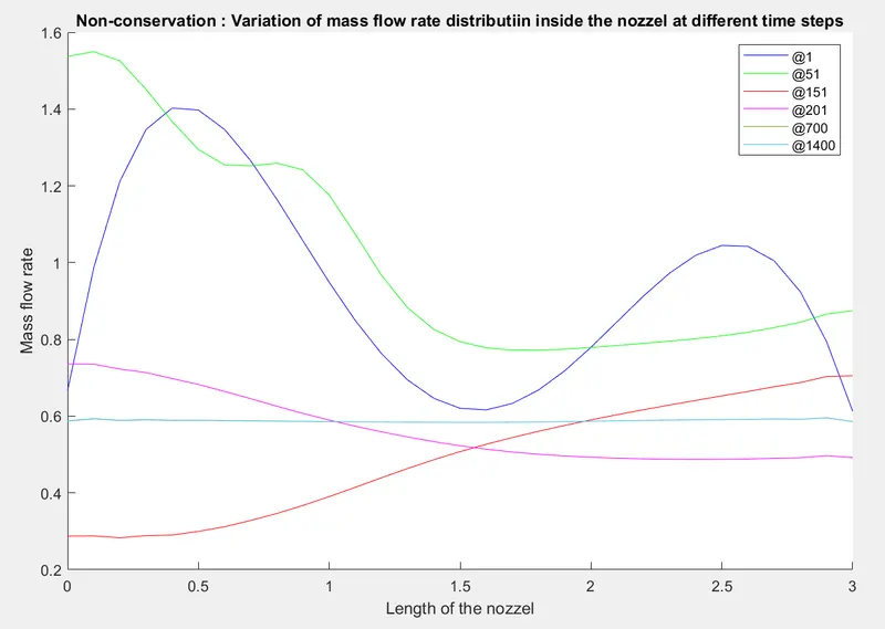
Variation of mass flow rate inside the nozzle at different time steps -
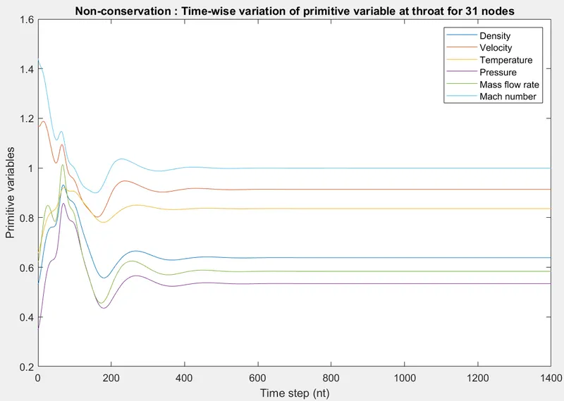
Time wise variation of primitive variables at the throat -
CONSERVATIVE FORM FUNCTION -
function [rho,T,v,mfr,mfr_throat] = conservation_form(n,l,nt,c,a,throat)

% Grid
x = linspace(0,l,n);
dx = x(2) - x(1);

g = 1.4;

for i = 1:length(x)

    if x(i) <= 0.5
        rho(i) = 1;
        T(i) = 1;
    elseif x(i) > 0.5 && x(i) <= 1.5
        rho(i) = 1 - 0.366*(x(i) - 0.5);
        T(i) = 1 - 0.167*(x(i) - 0.5);
    elseif x(i) > 1.5 && x(i) <= 3.5
        rho(i) = 0.634 - 0.3879*(x(i) - 1.5);
        T(i) = 0.833 - 0.3507*(x(i) - 1.5);
    end
end

% Solution vectors
u1 = rho.*a ;
v = (0.59)./u1 ;
u2 = rho.*a.*v ;
u3 = rho.*(T/(g-1) + (g/2)*(v.^2)).*a ;

% Initial values
mfr = (rho.*a).*v ;
mach_no = v./(sqrt(T)) ;

for i = 1:n
    dt = min((c*dx)./(sqrt(T(i)) + v(i)));
end

for k = 1:nt

    u1old = u1 ;
    u2old = u2 ;
    u3old = u3 ;

    % Flux vectors
    f1 = u2 ;
    f2 = ((u2.^2)./u1) + (((g-1)/g).*(u3 - ((g/2).*((u2.^2)./u1)))) ;
    f3 = g.*((u2.*u3)./u1) - (((g*(g-1))/2).*((u2.^3)./(u1.^2)));

    % Predictor step

    for i = 2:n-1

        % Source term
        j(i) = (1/g)*rho(i)*T(i)*((a(i+1)-a(i))/dx) ;

        % Continutiy equation
        du1_dt_p(i) = -((f1(i+1) - f1(i))/dx) ;

        % Momentum equation
        du2_dt_p(i) = -((f2(i+1) - f2(i))/dx) + j(i) ;

        % Energy equation
        du3_dt_p(i) = -((f3(i+1) - f3(i))/dx) ;

        % Solution vector update
        u1(i) = u1old(i) + du1_dt_p(i)*dt ;
        u2(i) = u2old(i) + du2_dt_p(i)*dt ;
        u3(i) = u3old(i) + du3_dt_p(i)*dt ;

    end

    % Flux vectors update
    f1 = u2 ;
    f2 = ((u2.^2)./u1) + (((g-1)/g).*(u3 - ((g/2).*((u2.^2)./u1)))) ;
    f3 = g.*((u2.*u3)./u1) - (((g*(g-1))/2).*((u2.^3)./(u1.^2)));

    % Corrector step

    for i = 2:n-1

        % Source term
        j(i) = (1/g)*rho(i)*T(i)*((a(i)-a(i-1))/dx) ;

        % Continutiy equation
        du1_dt_c(i) = -((f1(i) - f1(i-1))/dx) ;

        % Momentum equation
        du2_dt_c(i) = -((f2(i) - f2(i-1))/dx) + j(i) ;

        % Energy equation
        du3_dt_c(i) = -((f3(i) - f3(i-1))/dx) ;

    end

    % Computing the avaerage time derivative

    du1_dt = 0.5*(du1_dt_p + du1_dt_c) ;
    du2_dt = 0.5*(du2_dt_p + du2_dt_c) ;
    du3_dt = 0.5*(du3_dt_p + du3_dt_c) ;

    % Finale solution update

    for i = 2:n-1
        u1(i) = u1old(i) + du1_dt(i)*dt ;
        u2(i) = u2old(i) + du2_dt(i)*dt ;
        u3(i) = u3old(i) + du3_dt(i)*dt ;
    end

    % Decoding premitive variable values from solution vector

    rho = (u1)./(a) ;
    v = (u2)./(u1) ;
    T = (g-1)*((u3./u1) - (g/2)*(v.^2)) ;
    pressure = rho.*T  ;
    mfr = (rho.*a).*v ;
    mach_no = (v)./(sqrt(T)) ;

    % Apllying boundry conditions

    % Inlet
    u1(1) = rho(1)*a(1) ;
    u2(1) = 2*u2(2) - u2(3);
    u3(1) = u1(1).*((T(1)./(g-1)) + (g/2).*(v(1).^2)) ;

    % Outlet
    u1(n) = 2*u1(n-1) - u1(n-2);
    u2(n) = 2*u2(n-1) - u2(n-2);
    u3(n) = 2*u3(n-1) - u3(n-2);

    % Flow filed variables at throat

    rho_throat(k) = rho(throat);
    v_throat(k) = v(throat);
    T_throat(k) = T(throat);
    pressure_throat(k) = pressure(throat);
    mfr_throat(k) = mfr(throat);
    mn_throat(k) = mach_no(throat);

    if n == 31
        figure(4)
        hold on
        if k == 1
            plot(x,mfr,'b')
            title('Conservation : Variation of mass flow rate distributiin inside the nozzel at different time steps for 31 nodes')
        elseif k == 51
            plot(x,mfr,'g')
        elseif k == 151
            plot(x,mfr,'r')
        elseif k == 201
            plot(x,mfr,'m')
        elseif k == 700
            plot(x,mfr)
        elseif k == 1400
            plot(x,mfr)
            xlabel('Length of the nozzel')
            ylabel('Mass flow rate')
            legend('@1','@51','@151','@201','@700','@1400')
        end
    end

end

if n == 31
    figure(5)
    subplot(4,1,1)
    plot(x,v)
    title('Conservation : Steady State Distribution Of Primitive Variables for 31 nodes')
    ylabel('Velocity')
    grid on
    subplot(4,1,2)
    plot(x,T)
    ylabel('Temperature')
    grid on
    subplot(4,1,3)
    plot(x,rho)
    ylabel('Density')
    grid on
    subplot(4,1,4)
    plot(x,mach_no)
    ylabel('Mach Number')
    xlabel('Nozzel Length')
    grid on

    h = linspace(0,nt,nt);

    figure(6)
    plot(h,rho_throat);
    title('Conservation : Time-wise variation of primitive variable at throat for 31 nodes')
    hold on
    plot(h,v_throat);
    plot(h,T_throat);
    plot(h,pressure_throat);
    plot(h,mfr_throat);
    plot(h,mn_throat);
    legend('Density','Velocity','Temperature','Pressure','Mass flow rate','Mach number')
    xlabel('Time step (nt)')
    ylabel('Primitive variables')
    hold off
end

end
RESULTS FOR CONSERVATIVE FORM -
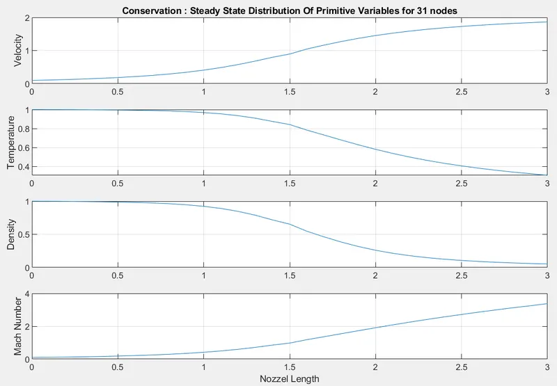
Steady state distribution of primitive variables -
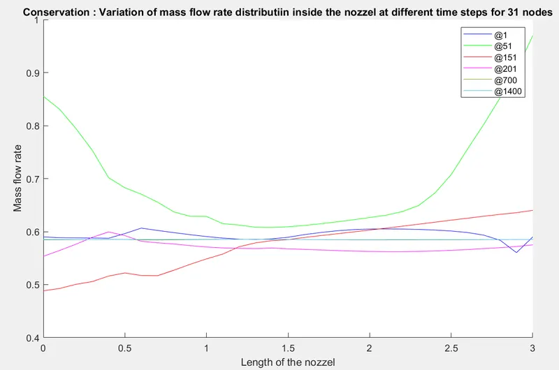
Variation of mass flow rate inside the nozzle at different time steps -
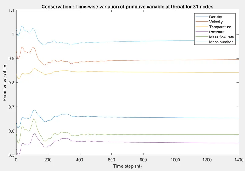
Time wise variation of primitive variables at the throat -
CONSERVATIVE Vs NON-CONSERVATIVE FORM -
Mass flow rate comparison at the throat and along the nozzle -
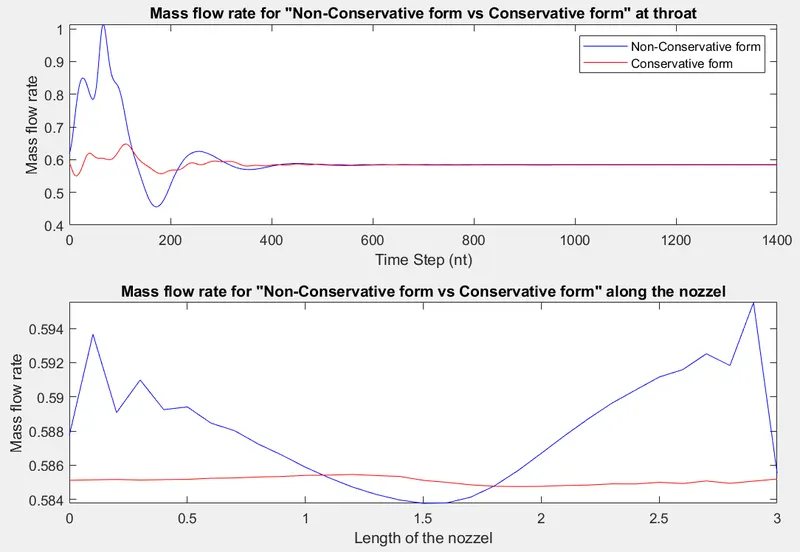
As we can see from the above plot, the variation of the mass flow rate at the throat is less for conservative form whereas for non-conservative form there's a large variation. The conservative form also achieves stability faster as compared to the non-conservative form.
We can also see that mass flow rate along the nozzle for conservative form is very stable as compared to non-conservative form in which there is lot of fluctuations.
GRID INDEPENDENCY TEST -
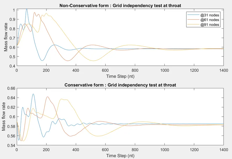
At throat -
Along the nozzle -
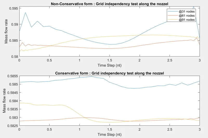
As we can see that for all the three grid sizes, if we select sufficient number of time steps all the three cases achieve stable solution and hence our solution is grid independent.
CONCLUSSION -
From the above study we can conclude that for both conservative and non-conservative form, we achieve convergence and stable solution. But looking at the graphs we can say that the conservative form gives a better, accurate and a smother result as compared to non-conservative form in which there's lots of fluctuation before achieving the stable solution.