Week 5.1 - Mid term project - Solving the steady and unsteady 2D heat conduction problem

OBJECTIVE – To solve 2D heat conduction equation for both steady state and transient state using implicit approach for the former one and both implicit and explicit approach for the latter one.

PROBLEM STATEMENT –

1. A square computational domain.
2. Number of nodes in x direction (nx) = Number of nodes in y direction(ny) = 10.
3. BOUNDARY CONDITIONS –
   Bottom boundary – 900k
   Top boundary – 600k
   Left boundary – 400k
   Right boundary – 800k
4. Initializing all other nodes with a random value (300k in our case).

THEORY – Heat conduction equation is a PDE that describes how heat is distributed through a domain as the time progresses.

General form of heat conduction equation is -

`(∂T)/(∂t)=α{(∂^2 T)/(∂x^2 )+(∂^2 T)/(∂y^2 )+ (∂^2 T)/(∂z^2 ) }`

Where T = Temperature function T(x,y,z,t)

`α` = thermal diffusivity of the medium (positive constant)

For our case, we’re only going to deal with 2D heat conduction equation which is given as

`(∂T)/(∂t)=α{(∂^2 T)/(∂x^2 )+(∂^2 T)/(∂y^2 )}`

In order to solve any PDE, there are two schemes namely Implicit and explicit schemes which can be used.

Let’s first discretize the 2D heat conduction equation. Since the RHS term, Laplacian of the temperature, is an elliptical nature PDE, we’ll have to take the information from all the points and hence we’ll use central difference method in both x and y direction.

The discretized PDE can be represented in two forms

• EXPLICIT FORM – `T_(i,j)^(n+1) = T_(i_, j)^n + (αΔt)( (T_L^(n)-2T_P^(n)+ T_R^(n))/(Δx^2) + (T_B^(n)-2T_P^(n)+ T_T^(n))/(Δy^2))`

• IMPLICIT FORM – `(T_(i,j)^(n+1)-T_(i_, j)^n)/(Δt) = α ((T_L^(n+1)-2T_P^(n+1)+ T_R^(n+1))/(Δx^2) + (T_B^(n+1)-2T_P^(n+1)+ T_T^(n+1))/(Δy^2))`
  
  

To solve an Explicit equation, we can use the time marching method in which we use previous time step values to compute present time step values and so on.

But to solve an Implicit equation, we can either form a matrix equation and then solve that equation. But using this matrix method is very length and difficult if there are large number of nodes and hence, we can use a solver known as iterative solver.

There are three types of iterative solver we’ll be looking at as given below

• Jacobi method
• Gauss-Seidel method
• Successive Over-Relaxation method (SOP)

STEADY STATE IMPLICIT APRROCH –

By using steady state, the above PDE reduces to only RHS as the time dependent terms becomes zero.

The steady state equation is given as

`(∂^2 T)/(∂x^2 )+(∂^2 T)/(∂y^2 )=0`

Now we can discretize this equation to solve it using implicit method

The discretized equation is given as

`(T_L^(n+1)-2T_P^(n+1)+ T_R^(n+1))/(Δx^2 ) + (T_B^(n+1)-2T_P^(n+1)+ T_T^(n+1))/(Δy^2 )=0`

Rearranging and simplifying the above equation give us

`T_P^(n+1) = 1/k {(T_L^(n+1)+ T_R^(n+1))/(Δx^2 ) + (T_B^(n+1)+ T_T^(n+1))/(Δy^2) }`

Where

`k = (2(Δx^2 + Δy^2))/(Δx^2*Δy^2 )`

Now we can write a code to solve the above equation.

MAIN MATLAB CODE FOR STEADY STATE IMPLICIT APPROCH -

clear all
close all
clc

% Inputs
n = 10;
T = 300*ones(n,n);

% Boundary conditions
T(1,:) = 900;
T(end,:) = 600;
T(:,end) = 800;
T(:,1) = 400;
T(1,1) = 650;
T(1,n) = 850;
T(n,1) = 500;
T(n,n) = 700;
Told = T;

% Defining the number of nodes in x and y direction
x = linspace(0,1,n); % Number of nodes in x direciton
dx = x(2) - x(1);
y = linspace(0,1,n); % Number of nodes in x direciton
dy = y(2) - y(1);

iterative_solver = 3; % 1 = jacobi solver, 2 = Gauss-seidel method, 3 = SOP method
error = 10; % Giving a random starting value for error
tol = 1e-4; % Tolerance value
k = (2*(dx^2 + dy^2))/((dx^2)*(dy^2)); % Constant used in the discretized equation.

if iterative_solver == 1  % Calling jacobi solver
[T,J_ite] = jacobi_steady_state_impl(error,tol,n,T,x,y,k,dx,dy);
end

if iterative_solver == 2  % Calling gauss-seidel solver
[T,GS_ite] = gs_steady_state_impl(error,tol,n,T,x,y,k,dx,dy);
end

if iterative_solver == 3  % Calling SOP solver
[T,SOP_ite] = sop_steady_state_impl(error,tol,n,T,x,y,k,dx,dy);
end

I have defined three function for three different method used in the above code, the function are as follows -

JACOBI SOLVER FUNCTION (STEADY STATE, IMPLICIT) -

function [T,jacobi_iter] = jacobi_steady_state_impl(error,tol,n,T,x,y,k,dx,dy)

Told = T; % Storing initial temperature values to use later.

%jacobi method

jacobi_iter = 1;

while(error > tol)  % Using while loop to check if the error is below the specified tolerance 
    for i = 2:n-1   % i = row number
        for j = 2:n-1  % j = column number 
            term1 = (Told(i-1,j) + Told(i+1,j))/(k*(dx^2));
            term2 = (Told(i,j-1) + Told(i,j+1))/(k*(dy^2));
            T(i,j) = term1 + term2;
        end
    end
    error = max(max(abs(Told-T))); % Updating error after every iteration
    Told = T;  % Updating the new temperature values so as to use them in next iteration
    jacobi_iter = jacobi_iter + 1; % Updating the iteration count after every iteration.
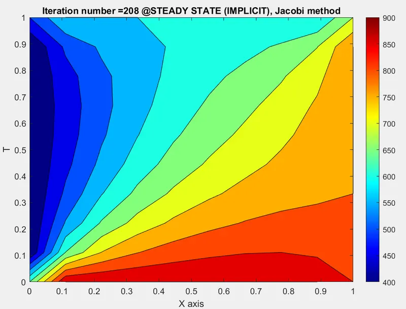
    contourf(x,y,T);
    colormap(jet)
    colorbar
    xlabel('X axis')
    ylabel('T')
    title_txt = sprintf('Iteration number =%d @STEADY STATE (IMPLICIT), Jacobi method',jacobi_iter);
    title(title_txt)
    pause(0.03)
end

RESULTS FOR JACOBI SOLVER (STEADY STATE , IMPLICIT) -

GAUSS SEIDEL SOLVER FUNCTION (STEADY STATE, IMPLICIT) -

function [T,gs_iter] = gs_steady_state_impl(error,tol,n,T,x,y,k,dx,dy)

Told = T; % Storing initial temperature values to use later.

%gs method

gs_iter = 1;

while(error > tol)  % Using while loop to check if the error is below the specified tolerance
    for i = 2:n-1   % i = row number
        for j = 2:n-1  % j = column number
            term1 = (T(i-1,j) + Told(i+1,j))/(k*(dx^2));
            term2 = (T(i,j-1) + Told(i,j+1))/(k*(dy^2));
            T(i,j) = term1 + term2;
        end
    end
    error = max(max(abs(Told-T)));  % Updating error after every iteration
    Told = T;  % Updating the new temperature values so as to use them in next iteration
    gs_iter = gs_iter + 1;  % Updating the iteration count after every iteration.
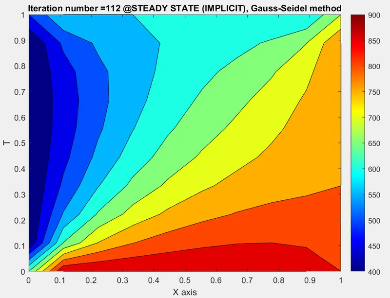
    contourf(x,y,T);
    colormap(jet)
    colorbar
    xlabel('X axis')
    ylabel('T')
    title_txt = sprintf('Iteration number =%d @STEADY STATE (IMPLICIT), Gauss-Seidel method',gs_iter);
    title(title_txt)
    pause(0.03)
end

RESULTS FOR GAUSS-SEIDEL SOLVER (STEADY STATE , IMPLICIT) -

SOP SOLVER FUNCTION (STEADY STATE, IMPLICIT) -

function [T,sop_iter] = sop_steady_state_impl(error,tol,n,T,x,y,k,dx,dy)

Told = T;  % Storing initial temperature values to use later.
w = 1.5; % Relaxation factor

%sop method

sop_iter = 1;

while(error > tol)  % Using while loop to check if the error is below the specified tolerance
    for i = 2:n-1   % i = row number
        for j = 2:n-1 % j = column number
            term1 = (T(i-1,j) + Told(i+1,j))/(k*(dx^2));
            term2 = (T(i,j-1) + Told(i,j+1))/(k*(dy^2));
            T(i,j) = Told(i,j)*(1-w) + w*(term1 + term2);
        end
    end
    error = max(max(abs(Told-T))); % Updating error after every iteration
    Told = T; % Updating the new temperature values so as to use them in next iteration
    sop_iter = sop_iter + 1; % Updating the iteration count after every iteration.
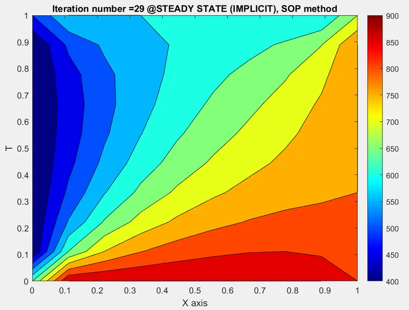
    contourf(x,y,T);
    colormap(jet)
    colorbar
    xlabel('X axis')
    ylabel('T')
    title_txt = sprintf('Iteration number =%d @STEADY STATE (IMPLICIT), SOP method',sop_iter);
    title(title_txt)
    pause(0.03)
end

RESULTS FOR SOP SOLVER (STEADY STATE , IMPLICIT) -

TRANSIENT STATE IMPLICIT APRROCH –

In transient state the main PDE eqaution does not changes and we can directly move on to dizcretize the PDE.

The discretized equation is given as

`(T_(i,j)^(n+1)-T_(i_, j)^n)/(Δt) = α( (T_L^(n+1)-2T_P^(n+1)+ T_R^(n+1))/(Δx^2) + (T_B^(n+1)-2T_P^(n+1)+ T_T^(n+1))/(Δy^2))`

Rearranging and simplifying the above equation give us

`T_P^(n+1)=k*T_p^n + (k*k1)*{T_L^(n+1)+ T_R^(n+1) } + (k*k2)*{T_T^(n+1)+ T_B^(n+1)}`

where `k= 1/(1 + 2k1 + 2k2 )` , `k1= α(Δt)/(Δx^2 )` , `k2= α(Δt)/(Δy^2 )`

Now we can move on to solve the above equation usinng the implicit method.

MAIN MATLAB CODE FOR TRANSIENT STATE IMPLICIT APPROCH -

clear all
close all
clc

% Inputs
n = 10;
T = 300*ones(n,n);

% Boundary conditions
T(1,:) = 900;
T(end,:) = 600;
T(:,end) = 800;
T(:,1) = 400;
T(1,1) = 650;
T(1,n) = 850;
T(n,1) = 500;
T(n,n) = 700;
Told = T;

% Defining the number of nodes in x and y direction
x = linspace(0,1,n);  % Number of nodes in x direciton
dx = x(2) - x(1);
y = linspace(0,1,n);  % Number of nodes in y direciton
dy = y(2) - y(1);
dt = 0.01;  % time step

iterative_solver = 3;  % 1 = jacobi solver, 2 = Gauss-seidel method, 3 = SOP method
error = 10;  % Giving a random starting value for error
tol = 1e-4;  % Tolerance value
alpha = 1.3; % Thermal diffusivity


if iterative_solver == 1  % Calling jacobi solver
[T,j_i] = jacobi_tran_state_impl(tol,n,T,x,y,dx,dy,alpha,dt);
end

if iterative_solver == 2  % Calling gauss-seidel solver
[T,gs_i] = gs_tran_state_impl(tol,n,T,x,y,dx,dy,alpha,dt);
end

if iterative_solver == 3  % Calling SOP solver
[T,sop_i] = sop_tran_state_impl(tol,n,T,x,y,dx,dy,alpha,dt);
end

I have defined three function for three different method used in the above code, the function are as follows -

JACOBI SOLVER FUNCTION (TRANSIENT STATE, IMPLICIT) -

function [T,jacobi_iter] = jacobi_tran_state_impl(tol,n,T,x,y,dx,dy,alpha,dt)

Told = T; % Storing initial temperature values to use later.
Told_p = Told;

k1 = (alpha*dt)/(dx^2);
k2 = (alpha*dt)/(dy^2);

%jacobi method

jacobi_iter = 1;

for s = 1:1400 % Time loop
    error = 900000;
    while(error > tol)   % Using while loop to check if the error is below the specified tolerance 
       for i = 2:n-1     % i = row number
           for j = 2:n-1 % j = column number
              term1 = 1/(1 + 2*k1 + 2*k2);
              term2 = k1*term1;
              term3 = k2*term1;
              H = (Told(i-1,j) + Told(i+1,j));
              V = (Told(i,j-1) + Told(i,j+1));
              T(i,j) = Told_p(i,j)*term1 + H*term2 + V*term3 ;
           end
       end
       error = max(max(abs(Told-T)));  % Updating error after every iteration
       Told = T;  % Updating the new temperature values so as to use them in next iteration
       jacobi_iter = jacobi_iter + 1;  % Updating the iteration count after every iteration.
    end
    Told_p = T;
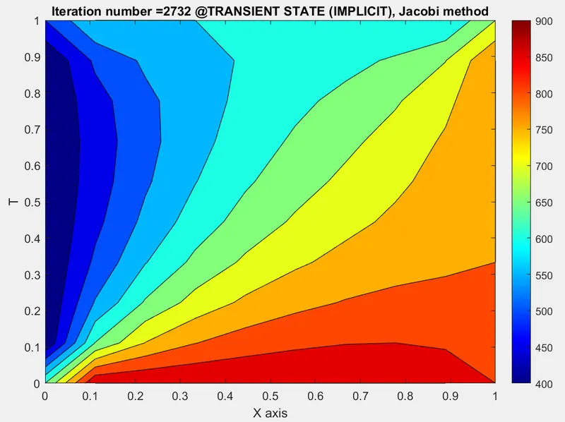
    contourf(x,y,T);
    colormap(jet)
    colorbar
    xlabel('X axis')
    ylabel('T')
    title_txt = sprintf('Iteration number =%d @TRANSIENT STATE (IMPLICIT), Jacobi method',jacobi_iter);
    title(title_txt)
    pause(0.03)
end

RESULTS FOR JACOBI SOLVER (TRANSIENT STATE , IMPLICIT) -

GUASS-SEIDEL SOLVER FUNCTION (TRANSIENT STATE, IMPLICIT) -

function [T,gs_iter] = gs_tran_state_impl(tol,n,T,x,y,dx,dy,alpha,dt)

Told = T; % Storing initial temperature values to use later.
Told_p = Told;

k1 = (alpha*dt)/(dx^2);
k2 = (alpha*dt)/(dy^2);

%gs method

gs_iter = 1;

for s = 1:1400  % Time loop
    error = 900000;
    while(error > tol)   % Using while loop to check if the error is below the specified tolerance 
       for i = 2:n-1     % i = row number
           for j = 2:n-1 % j = column number
              term1 = 1/(1 + 2*k1 + 2*k2);
              term2 = k1*term1;
              term3 = k2*term1;
              H = (T(i-1,j) + Told(i+1,j));
              V = (T(i,j-1) + Told(i,j+1));
              T(i,j) = Told_p(i,j)*term1 + H*term2 + V*term3 ;
           end
       end
       error = max(max(abs(Told-T)));   % Updating error after every iteration
       Told = T;  % Updating the new temperature values so as to use them in next iteration
       gs_iter = gs_iter + 1; % Updating the iteration count after every iteration.
    end
    Told_p = T;
    contourf(x,y,T);
    colormap(jet)
    colorbar
    xlabel('X axis')
    ylabel('T')
    title_txt = sprintf('Iteration number =%d @TRANSIENT STATE (IMPLICIT), Gauss-seidel method',gs_iter);
    title(title_txt)
    pause(0.03)
end

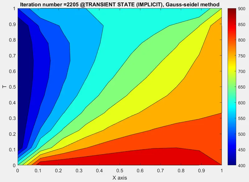
RESULTS FOR GUASS-SEIDEL SOLVER (TRANSIENT STATE , IMPLICIT) -

SOP SOLVER FUNCTION (TRANSIENT STATE, IMPLICIT) -

function [T,sop_iter] = sop_tran_state_impl(tol,n,T,x,y,dx,dy,alpha,dt)

Told = T; % Storing initial temperature values to use later.
Told_p = Told;

k1 = (alpha*dt)/(dx^2);
k2 = (alpha*dt)/(dy^2);
w = 1.2;

%sop method

sop_iter = 1;

for s = 1:1400 % Time loop
    error = 900000;
    while(error > tol)   % Using while loop to check if the error is below the specified tolerance 
       for i = 2:n-1     % i = row number
           for j = 2:n-1 % j = column number
              term1 = 1/(1 + 2*k1 + 2*k2);
              term2 = k1*term1;
              term3 = k2*term1;
              H = (T(i-1,j) + Told(i+1,j));
              V = (T(i,j-1) + Told(i,j+1));
              T(i,j) = Told(i,j)*(1-w) + w*(Told_p(i,j)*term1 + H*term2 + V*term3) ;
              
           end
       end
       error = max(max(abs(Told-T)));
       Told = T;
       sop_iter = sop_iter + 1;
    end
    Told_p = T;
    contourf(x,y,T);
    colormap(jet)
    colorbar
    xlabel('X axis')
    ylabel('T')
    title_txt = sprintf('Iteration number =%d @TRANSIENT STATE (IMPLICIT), SOP method',sop_iter);
    title(title_txt)
    pause(0.03)
end

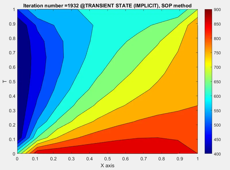
RESULTS FOR SOP SOLVER (TRANSIENT STATE , IMPLICIT) -

TRANSIENT STATE EXPLICIT APRROCH –

In transient state the main PDE eqaution does not changes and we can directly move on to dizcretize the PDE.

The discretized equation is given as

`T_(i,j)^(n+1) = T_(i_, j)^n + (αΔt)( (T_L^(n)-2T_P^(n)+ T_R^(n))/(Δx^2) + (T_B^(n)-2T_P^(n)+ T_T^(n))/(Δy^2))``

Now we can move on to solve the above equation using the explicit method.

MATLAB CODE FOR TRANSIENT STATE EXPLICIT APPROCH -

clear all
close all
clc

% Inputs
n = 10;
T = 300*ones(n,n);

% Boundary conditions
T(1,:) = 900;
T(end,:) = 600;
T(:,end) = 800;
T(:,1) = 400;
T(1,1) = 650;
T(1,n) = 850;
T(n,1) = 500;
T(n,n) = 700;
Told = T;

error = 9000;  % Giving a random starting value for error
tol = 1e-4;    % Tolerance value

% Defining the number of nodes in x and y direction
x = linspace(0,1,n);  % Number of nodes in x direciton
dx = x(2) - x(1);
y = linspace(0,1,n);  % Number of nodes in y direciton
dy = y(2) - y(1);
dt = 0.002;  % time step

alpha = 1.1; % Thermal diffusivity
k1 = (alpha*dt)/(dx^2);
k2 = (alpha*dt)/(dy^2);
counter = 1; % Iteration counter

while(error>tol)    % Using while loop to check if the error is below the specified tolerance
    for i = 2:n-1   % i = row number
           for j = 2:n-1  % j = column number
               term1 = Told(i,j);
               term2 = k1*(Told(i-1,j) - 2*Told(i,j) + Told(i+1,j));
               term3 = k2*(Told(i,j-1) - 2*Told(i,j) + Told(i,j+1));
               T(i,j) = term1 + term2 + term3;
           end
    end
    counter = counter + 1; % Updating the iteration count after every iteration.
    error = max(max(abs(Told-T)));  % Updating error after every iteration
    Told = T; % Updating the new temperature values so as to use them in next iteration
    contourf(x,y,T);
    colormap(jet)
    colorbar
    xlabel('X axis')
    ylabel('T')
    title_txt = sprintf('Iteration number =%d @Transient state explicit',counter);
    title(title_txt)
    pause(0.03)
end

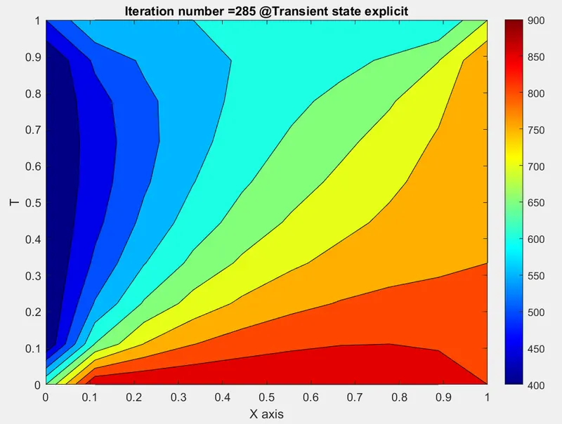
RESULTS (TRANSIENT STATE , EXPLICIT) -

RESULT INTERPRETATION -

Type of analysis and scheme comparison table -

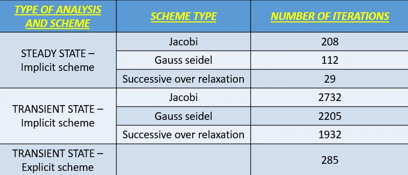
• As we can see from the above table, the greatest number of iterations need for convergence is in transient state analysis using implicit approach.
• 
  We can also see that number of Jacobi iteration > Gauss-seidel iterations > Successive over relaxation (SOP) iteration. This implies that we can use SOP method in order to improve the convergence of both Jacobi and Gauss-seidel method.
• 
  We can also see from the result plots that the result is same for both the analysis, steady state analysis and transient state analysis, that is because any system which starts as with transient state will always try and achieve the steady state and hence final answer for both the analysis is same.