Week 3.5 - Deriving 4th order approximation of a 2nd order derivative using Taylor Table method

OBJECTIVE – To drive and write a MATLAB program for 4^th order approximation of 2^nd order derivative of the function f(x) = exp(x)*cos(x) by following methods

1. Central difference method
2. Right-sided difference method
3. Left-sided difference method

THEORY - In order to solve any PDE, we first need to discretise the PDE in order to reduce the complicity to solve the PDE for continuous domain and rather solve for discrete points. To discretize any PDE there are three types of method, which are listed above.

CENTRAL DIFFERENCE METHOD –

The central difference method is a method in which we choose the nodes symmetrical to the specified point, that is we choose nodes from both sides of the specified point as shown below

(i-2)……….(i-1)……….(i)……….(i+1)……….(i+2)

Here i is the specified point and as we can se we’re choosing points from both sides of the i and hence this method is known as central difference method.

Formula for 4^th order approximation of 2^nd order derivative of a function f at x = i is given as

`(a*f(x-2dx)+b*f(x-dx)+c*f(x)+d*f(x+dx)+e*f(x+2dx))/(∇x^2 )= (d^2 f)/(dx^2 )`

We know need to find all the coefficients (a, b, c….) using the Taylor’s table method

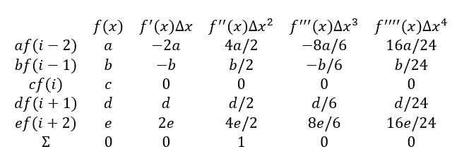
From the above table we can form 5 equations and solve them on MATLAB in order to get the values of a, b, c, d and e.

5 equations to solve are -

1. a + b + c + d + e = 0
2. -2a - b + 0 + d + 2e = 0
3. 4a/2 + b/2 + 0 + d/2 + 4e/2 = 1
4. -8a/6 - b/6 + 0 + d/6 + 8e/6 = 0
5. 16a/24 + b/24 + 0 + d/24 + 16e/24 = 0

MATLAB FUNCTION FOR CENTRAL DIFFERENCE METHOD

function [X] = central_diff()

%CENTRAL DIFFERENCE METHOD USING FOR LOOP FOR SIMPLICITY
b = [-2,-1,0,1,2]; % Nodes used in central difference method
d = [0;0;1;0;0];   % Summation output for different orders of derivative
n = length(b);
A = zeros(n,n);  % A matrix for storing coefficients of each derivatives

for i = 1:n       % For loop to calucate coefficients of each derivative of each node point
    for j = 1:n
        A(i,j) = ((b(i))^(j-1))/factorial(j-1);
    end
end
X = linsolve(A',d); % Using inbuilt matlab command to solve matrix equation to get values of a,b,c....

end

RIGHT-SIDED DIFFERENCE METHOD –

The right-sided difference method is a method in which we choose the nodes asymmetrical to the specified point, that is we choose nodes from only right side of the specified point as shown below

(i)……….(i+1)……….(i+2)……….(i+3)……….(i+4)……….(i+5)

Here i is the specified point and as we can see we’re choosing points only from right side of the i and hence this method is known as right-sided difference method.

Formula for 4^th order approximation of 2^nd order derivative of a function f at x = i is given as

`(a*f(x)+b*f(x+dx)+c*f(x+2dx)+d*f(x+3dx)+e*f(x+4dx)+g*f(x+5dx))/(∇x^2 )= (d^2 f)/(dx^2 )`

We know need to find all the coefficients (a, b, c….) using the Taylor’s table method

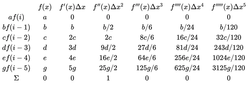
From the above table we can form 6 equations and solve them on MATLAB in order to get the values of a, b, c, d, e and g.

6 equations to solve are -

1. a + b + c + d + e + g = 0
2. 0 + b +2c + 3d + 4e + 5g = 0
3. 0 + b/2 +2c/6 + 9d/2 + 16e/2 + 25g/2 = 0
4. 0 + b/6 +8c/6 + 27d/6 + 64e/6 + 125g/6 = 0
5. 0 + b/24 +16c/24 + 81d/24 + 256e/24 + 625g/24 = 0
6. 0 + b/120 +32c/120 + 243d/120 + 1024e/120 + 3125g/120 = 0

MATLAB FUNCTION FOR RIGHT-SIDED DIFFERENCE METHOD

function [Y] = right_sided()

%SKEWED RIGHT-SIDED DIFFERENCE METHOD USING FOR LOOP FOR SIMPLICITY

b = [0,1,2,3,4,5];  % Nodes used in Right-sided difference method
d = [0;0;1;0;0;0];  % Summation output for different orders of derivative
n = length(b);
A = zeros(n,n);   % A matrix for storing coefficients of each derivatives

for i = 1:n         % For loop to calucate coefficients of each derivative of each node point
    for j = 1:n
        A(i,j) = ((b(i))^(j-1))/factorial(j-1);
    end
end
Y = linsolve(A',d); % Using inbuilt matlab command to solve matrix equation to get values of a,b,c....

end

LEFT-SIDED DIFFERENCE METHOD –

The left-sided difference method is a method in which we choose the nodes asymmetrical to the specified point, that is we choose nodes from only left side of the specified point as shown below

(i-5)……….(i-4)……….(i-3)……….(i-2)……….(i-1)……….(i)

Here i is the specified point and as we can see we’re choosing points only from left side of the i and hence this method is known as right-sided difference method.

Formula for 4^th order approximation of 2^nd order derivative of a function f at x = i is given as

`(a*f(x)+b*f(x-dx)+c*f(x-2dx)+d*f(x-3dx)+e*f(x-4dx)+g*f(x-5dx))/(∇x^2 )= (d^2 f)/(dx^2 )`

We know need to find all the coefficients (a, b, c….) using the Taylor’s table method

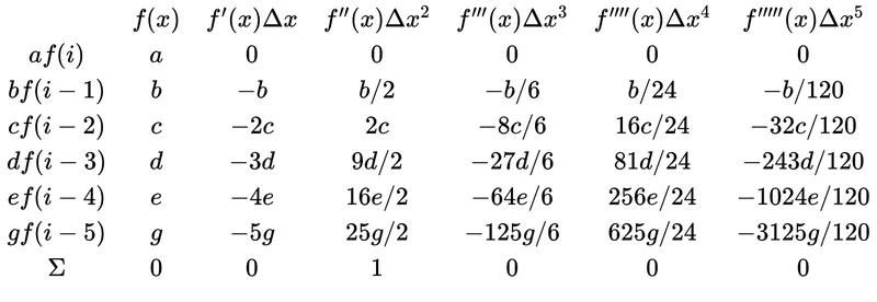
From the above table we can form 6 equations and solve them on MATLAB in order to get the values of a, b, c, d, e and g.

6 equations to solve are -

1. a +b +c +d +e +g = 0
2. 0 -b -2c -3d -4e -5g = 0
3. 0 +b/2 +2c/6 +9d/2 +16e/2 +25g/2 = 0
4. 0 -b/6 -8c/6 -27d/6 -64e/6 -125g/6 = 0
5. 0 +b/24 +16c/24 +81d/24 +256e/24 +625g/24 = 0
6. 0 -b/120 -32c/120 -243d/120 -1024e/120 -3125g/120 = 0

MATLAB CODE FOR LEFT-SIDED DIFFERENCE METHOD

function [Z] = left_sided()

%SKEWED LEFT-SIDED DIFFERENCE  METHOD USING FOR LOOP FOR SIMPLICITY

b = [0,-1,-2,-3,-4,-5];  % Nodes used in Left-sided difference method
d = [0;0;1;0;0;0];       % Summation output for different orders of derivative
n = length(b);
A = zeros(n,n);        % A matrix for storing coefficients of each derivatives

for i = 1:n              % For loop to calucate coefficients of each derivative of each node point
    for j = 1:n
        A(i,j) = ((b(i))^(j-1))/factorial(j-1);
    end
end

Z = linsolve(A',d);  % Using inbuilt matlab command to solve matrix equation to get values of a,b,c....

end

Since we're done with finding the equations and there solutions using matlab, we can now move forward to writing code to compare there errors.

MATLAB CODE FOR ERROR COMPARISON -

clear all
close all
clc

X = central_diff ;  % Central difference function
Y = right_sided ;   % Right-sided difference function
Z = left_sided ;    % Left-sided difference function

% Now as we're done with getting formuls for all the three methods, we can now move on to calculate 
% the error and compare error by each method.

x = pi/3 ; %specified point for derivate calculation.
dx = linspace(pi/4,pi/400,20) ; %specified time step range.
n = length(dx);

f = @(x) exp(x)*cos(x); % using anonymous function to specify the function for simplicity.

analytical_derivative = -2*exp(x)*sin(x);

for i = 1:n % Using for loop to calculate error at each time set

central_difference(i) = (X(1)*f(x-2*dx(i)) + X(2)*f(x-dx(i)) + X(3)*f(x) + X(4)*f(x+dx(i)) + X(5)*f(x+2*dx(i)))/((dx(i))^2);

right_sided_diff(i) = (Y(1)*f(x) + Y(2)*f(x+dx(i)) + Y(3)*f(x+2*dx(i)) + Y(4)*f(x+3*dx(i)) + Y(5)*f(x+4*dx(i)) + Y(6)*f(x+5*dx(i)))/((dx(i))^2);

left_sided_diff(i) = (Z(1)*f(x) + Z(2)*f(x-dx(i)) + Z(3)*f(x-2*dx(i)) + Z(4)*f(x-3*dx(i)) + Z(5)*f(x-4*dx(i)) + Z(6)*f(x-5*dx(i)))/((dx(i))^2);

% Using absolute value so that the answer doesn't change even if we change the order during substraction. 

error1(i) = abs(analytical_derivative - central_difference(i)); % 1st order approximation error.

error2(i) = abs(analytical_derivative - right_sided_diff(i)); % 2nd order approximation error.

error3(i) = abs(analytical_derivative - left_sided_diff(i)); % 4th order approximation error.

end

%Using Log plot of dx vs error for better understanding the reslut since our values are really small 
%and hence its difficult to see the change in error with time.

loglog(dx,error1,'linewidth',3) % log plot for 1st order approximation
hold on 
loglog(dx,error2,'linewidth',3) % log plot for 2nd order approximation
loglog(dx,error3,'linewidth',3) % log plot for 4th order approximation
hold off
title('4th order approximation of 2nd order derivative by different ways')
legend('Central difference','Right-Sided difference','Left-Sided difference')
xlabel('dx')
ylabel('Truncation error')

WHY WE'RE USING LOG PLOT

We are using log plot to show dx vs error because the error values are very small and in a regular plot it’s difficult to visualize the result and hence difficult to make any interpretation from regular plot. Log plot gives a better visualization and hence helps in interpretating the result.

LOG PLOT (result)

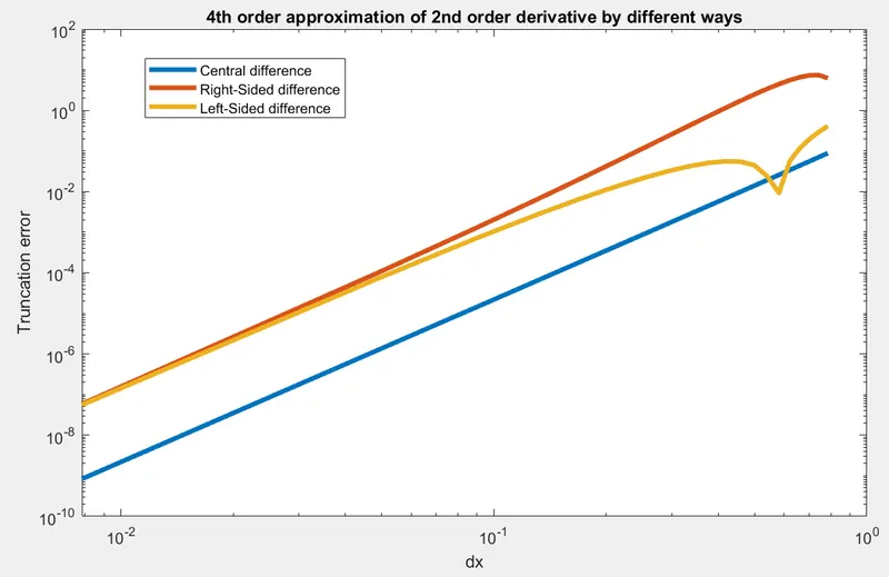
Result interpretation

1. As we can see from the above plot, the truncation error is almost same for both skewed right-sided difference and skewed left-sided difference for small grid size (dx).
2. 
   We can also see that for a given grid size (dx), truncation error for central difference is less as compared to both skewed right-sided difference and skewed left-sided difference, hence central difference method is better for error reduction.
3. 
   Since central difference method takes information from both right and left side point, this method is not suited for boundary value problem as there's not enough points present for its calculations. Hence in many problems skewed difference method is used because of its skewed nature.