Week 6 - CHT Analysis on a Graphics card

Assignment Name- CHT on graphics card

Aim- perform simulation of CHT on Graphics Card with varying velocities and calculate heat transfer coefficient

Objective-

1. Run the simulation by varying the velocity from 1m/sec to 5m/sec for at least 3 velocities and discuss the results.
2. Find out the maximum temperature and heat transfer coefficient attained by the processor.
3. Prove that the simulation has achieved convergence with appropriate images and plots.
4. Identify potential hotspots on the mode

Conjugate heat transfer:

The Conjugate Heat Transfer (CHT) analysis type allows for the simulation of heat transfer between solid and fluid domains by exchanging thermal energy at the interfaces between them. Typical applications of this analysis type exist as, but are not limited to, the simulation of heat exchangers, cooling of electronic equipment, and general-purpose cooling and heating systems.

e.g

HVAC, Heat Exchanger, Tank, Internal Combustion Engine, Heat Sink, Boiler, Reactor, Heat Pipe, Turbocharger.

Heat Transfer in a Solid - Conduction: Diffusion of heat due to temperature gradients in solids. A measure of the amount of conduction for a given gradient is heat conductivity. Conduction is described by Fourier’s law defining the conductive heat flux, q, proportional to the temperature gradient

Heat Transfer in a Fluid - Convection: When heat is carried away by moving fluid. The flow can either be caused by external influences, forced convection or by buoyancy forces, natural convection.

Due to the fluid motion, there are three contributions to the heat transfer:

Convective contribution: Depending on the properties of the fluid and its region of flow, the domination of conduction and convection varies.

Viscous effects: Due to the fluid flow, the viscosity creates heat. This effect is often neglected due to its negligible value but should be taken into account for high-velocity cases.

Density effects: When the density becomes related to the temperature, the domain will have different densities at different locations based on the temperature distribution. This variation in density can cause the compression which in-turn generates the heat.

The contemporary conjugate convective heat transfer model was developed after computers came into wide use in order to substitute the empirical relation of proportionality of heat flux to temperature difference with heat transfer coefficient which was the only tool in theoretical heat convection since the times of Newton. This model, based on a strictly mathematically stated problem, describes the heat transfer between a body and a fluid flowing over or inside it as a result of the interaction of two objects. The physical processes and solutions of the governing equations are considered separately for each object in two subdomains. Matching conditions for these solutions at the interface provide the distributions of temperature and heat flux along the body–flow interface, eliminating the need for a heat transfer coefficient. Moreover, it may be calculated using these data.

Applications:

Starting from simple examples in the 1960s, the conjugate heat transfer methods have become a more powerful tool for modelling and investigating natural phenomena and engineering systems in different areas ranging from aerospace and nuclear reactors to thermal goods treatment and food processing, from complex procedures in medicine to atmosphere/ocean thermal interaction in meteorology, and from relatively simple units to multistage, nonlinear processes. A detailed review of more than 100 examples of conjugate modelling selected from a list of 200 early and modern publications shows that conjugate methods are now used extensively in a wide range of applications. That also is confirmed by numerous results published after this book appearance (2009) that one may see, for example, at the Web of Science. The applications in specific areas of conjugate heat transfer at periodic boundary conditions and in exchanger ducts are considered in two recent books.

Simulations-steps involved for this simulation

Geometry

Mesh

Setup

Solution

Results

Geometry-

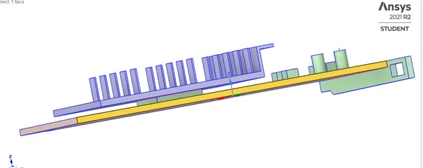
Step file is imported to space claim

There is total four parts namely like

Base

Fin-base

Processor

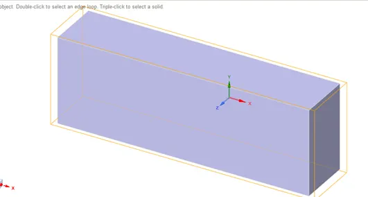
Encloser

Then share the topology is on for sharing information for purpose of conformal mesh to obtain accurate results

Mesh

Base line mesh

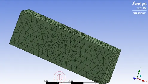
Default element size=10.289 mm

Number of elements=81932

Number of nodes=15466

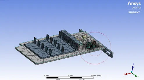
Refined Mesh

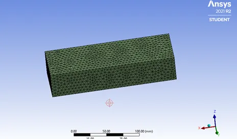
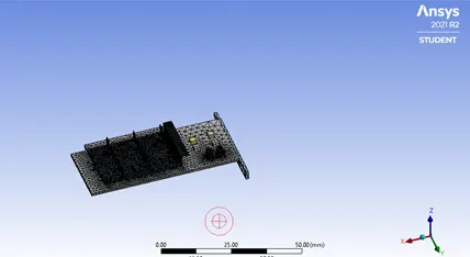
Element size=5 mm

Number of elements=369107

Number of nodes=64977

Sizing for fin=0.5 mm

Sizing for processor=0.5 mm

I am going for refined mesh for further calculations

I not go for more fine mesh than above because of restriction of student ANSYS software

setup-

solver type-pressure Based Solver-steady state

model-viscous k-epsilon standard

energy-turn on

boundary condition-

inlet velocity-1m/s

temperature-300k

outlet-pressure outlet

material properties

fluid-air

density=1.225 kg/m^3

specific heat (Cp)=1006.43 J/Kg k

thermal conductivity=0.0242 W/m k

viscosity=1.7894e-05

solid-

aluminium

density=2719 kg/m^3

specific heat (Cp)=871 J/Kg k

thermal conductivity=202.4 W/m k

copper

density=8978 kg/m^3

specific heat (Cp)=381 J/Kg k

thermal conductivity=387.6 W/m k

steel

density=8030 kg/m^3

specific heat (Cp)=502.48 J/Kg k

thermal conductivity=16.27 W/m k

cell zone conditions

fin-base set to solid-Aluminium

processor set to solid-copper

Base set to solid -steel

There is only processor is source term so consider

So internal heat generation=5e7 W/m^3

Volume of processor=8*8*1=64 mm^3

Heat generated per volume=heat generation/Volume of processor

Hence heat generated by processor =3.2 W (required for calculating heat transfer coefficient)

Method= coupled

Initialization-hybrid

Solutions-

For Velocity= 1 m/s

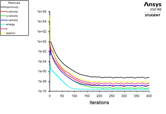
Residual plot

We assumed that solution is converge after 150-200 iterations because there is no change in residual plot

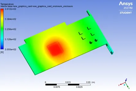
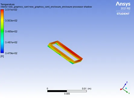
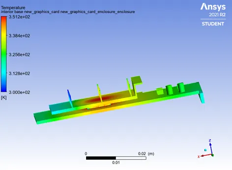
Temperature contour

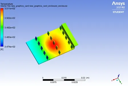
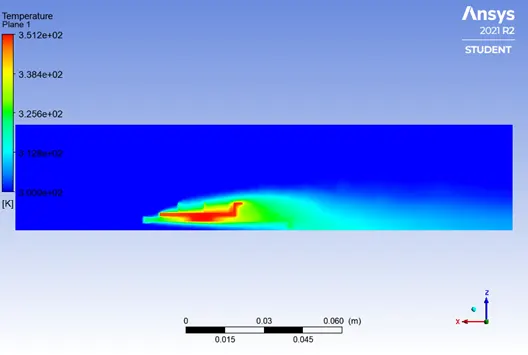
Temperature contour (plane)

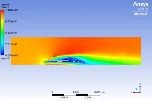
Velocity contour(plane)

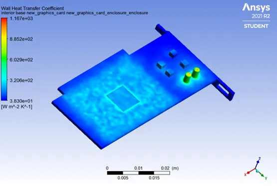
Wall heat transfer coefficient

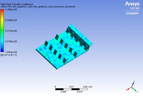
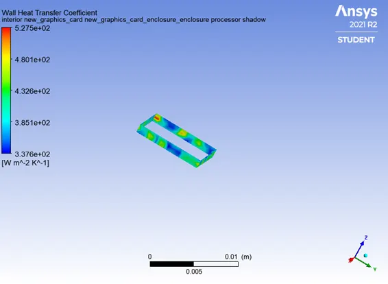
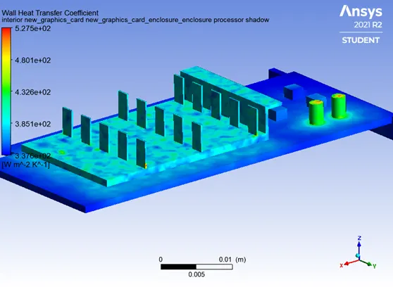
Wall heat transfer coefficient by inserting plane

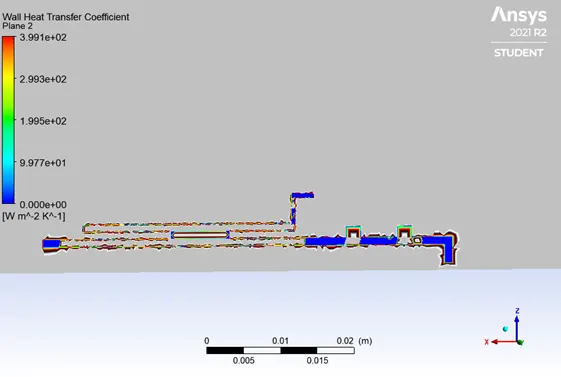
For Velocity= 3 m/s

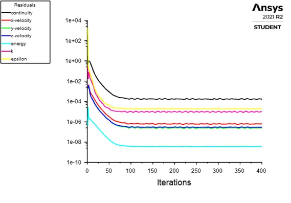
Residual plot

We assumed that solution is converge after 150-200 iterations because there is no change in residual plot

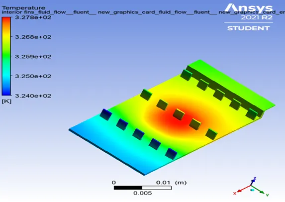
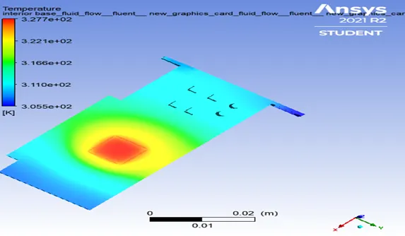
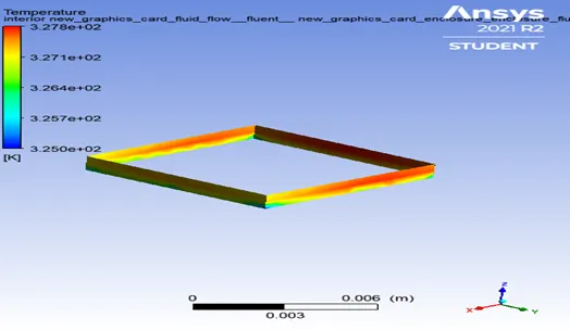
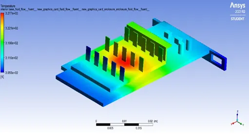
Temperature contour

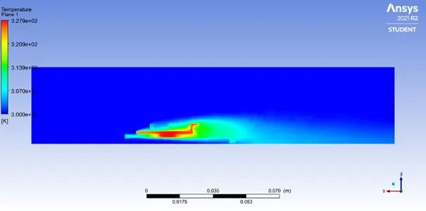
Temperature contour(plane)

Velocity Contour(plane)

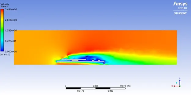
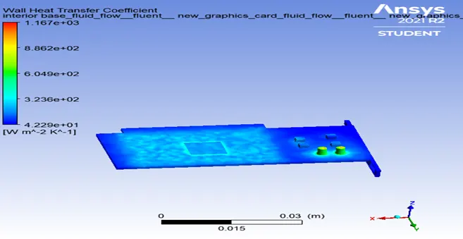
Wall heat transfer coefficient

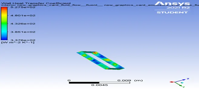
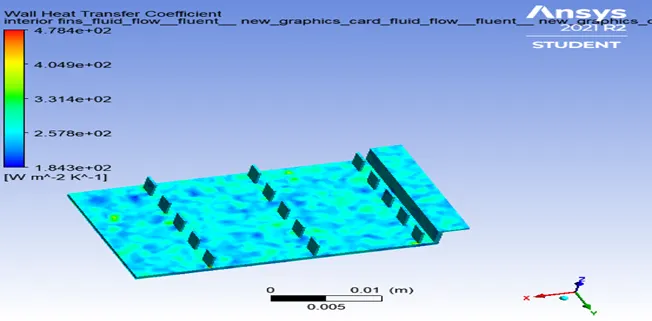
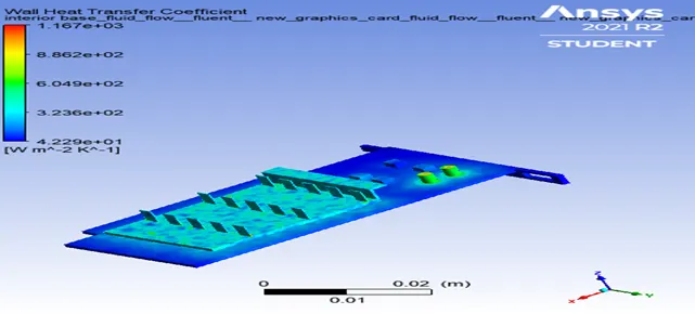
Wall heat transfer coefficient by inserting plane

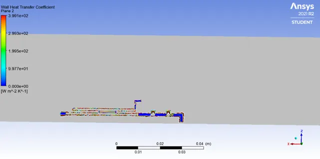
For Velocity= 5m/s

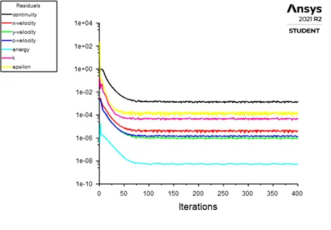
Residual plot

We assumed that solution is converge after 150 iterations because there is no change in residual plot

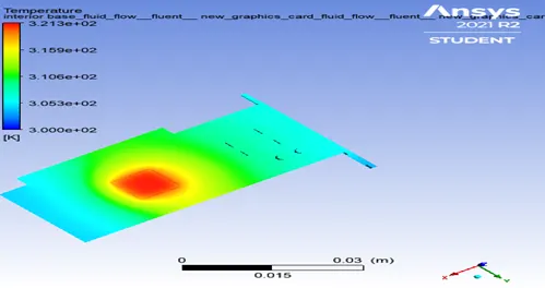
Temperature contour

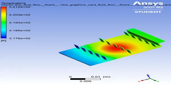
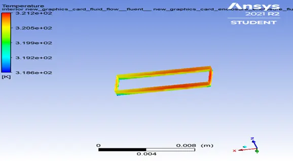
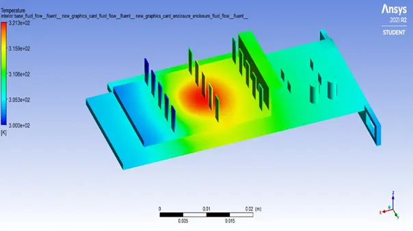
Temperature contour(plane)

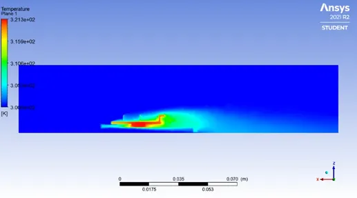
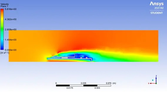
Velocity Contour(plane)

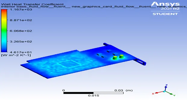
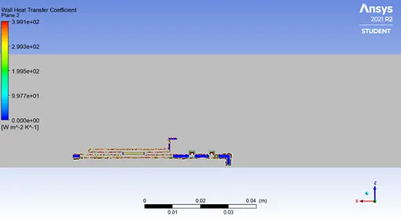
Wall heat transfer coefficient

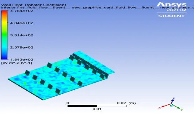
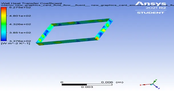
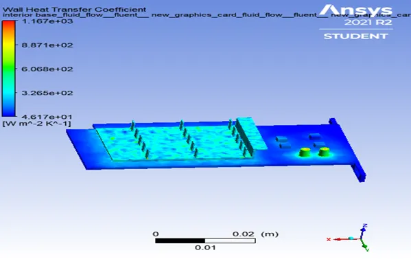
Wall heat transfer coefficient by inserting plane

Why particular material used for particular components

Copper-used as processor material-copper used as processor because of following characteristics

high electrical conductivity

Good heat conductivity

Corrosion resistances

Copper is used in electrical equipment’s

Aluminium- used as fins material

Good corrosion resistance

High thermal conductivity

For this characteristics aluminium used as material of fins

Steel-used as base material

Hardness

Tensile strength

Toughness

Corrosion resistance

Steel used as base material due to durability and soundproofing quantities

Other material also we can used in graphics card like gold, silver, nickel, silicon, tungsten etc.

Calculations

Q=h*A(T2-T1)

For v=1m/s

Q=3.2W ___- (for this we refer setup para)

Q/A=q (heat flux W/m^2)

h=heat transfer coefficient

T2=temperature of solid

T1=temperature of fluid

A=area of processor=2WL+2Lh+2HW=272*10^ ( -6 )

h=Q/A(T2-T1)

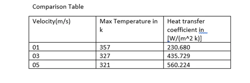
h=230.680 W/ (m^2 *k)

similarly calculate heat transfer coefficient for velocity at 3m/s,5m/s

at velocity 3m/s

h=435.729 W/(m^2 *k)

at velocity 5m/s

h=560.224W/(m^2 *k)

Comparison Table

Conclusions-

• Simulation at velocity=1m/s, 3m/s, 5m/s is converged

• Potential hotspot is seen near the area of processor which is getting heated up due to high temperature of processor
• We have known higher the velocity; higher the heat transfer Rate hence heat transfer coefficient increases with the increasing velocity so from above table of comparison we easily said that our simulation is validate
• As velocity increase ;temperature decrease