Conjugate heat transfer Analysis on a Graphics card
I. Aim: Numerical analysis of conjugate heat transfer of a graphics card.
II. Introduction:
Conjugate heat transfer (CHT) is the heat transfer mechanism occurring at a solid-fluid interface. This type of heat transfer includes both convection (fluid side) and conductive (solid side) heat transfer. The fluid side convection may be natural convection or due to forced convection.
The common examples of CHT are heat transfer between different fluids through heat exchangers, cooling of automobile engines with fins, heat sink applications in electronic equipment, electric motor cooling, and battery thermal management in Electric vehicles, etc. Forced convection on the fluid side plays an important role in achieving high heat transfer rates between the solid surface and the fluids.
Designing the optimum heat transfer interface between the solid surface and the heat transfer fluid plays an important role in keeping the electronic equipment, automobile engines, Electric vehicles, Industrial machinery at their operating temperatures, and better heat transfer in heat exchangers to maximize the performance efficiencies.
CHT analysis comes into the picture in designing the optimum heat transfer model for the above applications. Particularly, numerical CHT analysis using CFD plays an important role to design better heat transfer mechanisms. Using CHT analysis the optimum material and geometry for the solids as well as the flow rates and fluid properties can be realized for each application. The CHT analysis in CFD solves the convection physics on the fluid side and conduction physics on the solid side.
Fluid/Solid Interface heat interaction:
The temperature field and the heat flux are continuous at the fluid/solid interface. However, the temperature field can rapidly vary in a fluid in motion: close to the solid, the fluid temperature is close to the solid temperature, and far from the interface, the fluid temperature is close to the inlet or ambient fluid temperature. The distance where the fluid temperature varies from the solid temperature to the fluid bulk temperature is called the thermal boundary layer. The thermal boundary layer size and the momentum boundary layer relative size is reflected by the Prandtl number `Pr = (muC_p)/k`: for the Prandtl number to equal 1, thermal and momentum boundary layer thicknesses need to be the same. A thicker momentum layer would result in a Prandtl number larger than 1. Conversely, a Prandtl number smaller than 1 would indicate that the momentum boundary layer is thinner than the thermal boundary layer.
CHT Analysis of a Graphics card:
The graphics card is an essential component of the current generation computers and other smart devices to enhance the user experience in processing the images and video content. Due to the amount of data it processes in a short amount of time, a lot of heat is generated in the processor that degrades the performance of the processor if not dealt correctly. The performance of the graphics card (graphics processor) depends on its temperature. Heat has to be expelled from the processor to maintain it at its operating temperatures. Usually, a heat sink (fins) structure is attached to the processor to increase the surface area for enhancing heat dissipation. But this is not sufficient in high-end graphics processors and requires other cooling techniques. For this, forced convection is employed in the form of cooling liquid jackets or fans supplying ambient air to improve the heat removal from the processor and to maintain it at optimum temperature.
In this project, numerical CHT analysis of a typical graphics card of a computer, aided with cooling from forced convection with ambient air is carried in Ansys fluent software to study the conjugate heat transfer between the fluid (air) and the temperature distribution in the graphics card at three different fluid velocities between 1 to 5 m/s.
III Objectives:
- Run the simulation by varying the velocity from 1m/sec to 5m/sec for at least 3 velocities and discuss the results.
- Find out the maximum temperature and heat transfer coefficient attained by the processor.
- Prove that the simulation has achieved convergence with appropriate images and plots.
- Identify potential hotspots on the model.
IV: Solving & Modelling approach:
3D CFD analysis is carried out in Ansys workbench using Fluent solver to simulate the flow and conjugate heat transfer in the graphics card. Ambient air is used as the cooling fluid flowing around the graphics card.
V: Pre-processing and solver setting:
The first step in a CFD analysis is preprocessing. This includes preparing the geometry/ computational domain, discretization of the domain (meshing), assigning material properties, boundary conditions, solver setup.
1. Geometry/Domain:
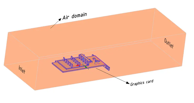
A 3D solid geometry of the typical graphics card is created in Spaceclaim. It consists of components like a processor which is the heat-generating component of the graphics card, a fin structure to increase the heat dissipation surface area, and a base to support the processor and fin structure. An enclosure is created around the graphics card to model the fluid domain. Further, share topology is enabled between the components as well as the fluid domain to have conformal mesh. The following figures show the processor, enclosed fluid (air) domain.
2. Domain discretization /Meshing:
The 3d fluid domain and the solid graphics card components are discretized into a finite number of control volumes using the Ansys meshing component. A 3D tetrahedral/hexahedral mesh is created for the graphics card and the fluid domain to accurately capture the geometry. Two different mesh were employed to check the effect of cell size on the results. The following table shows the mesh details:
| Property | Coarse Mesh | Refined mesh |
| Global element size | 4 mm | 2 mm |
| Body sizing - Processor | 3 mm | 2 mm |
| Cell count | 1,84,041 | 3,77,356 |
| Element quality | 0.82 | 0.83 |
The cell zones and boundaries of the domain are also defined in the Ansys mesher using the named selection option. The boundaries are defined as follows:
| Boundary/Cell Zone | Boundary/Cell Zone name |
| Inlet | inlet |
| Outlet | outlet |
| Fluid domain wall | domain walls |
| Fluid domain (fluid zone) | Air |
| Processor (solid zone) | processor |
| Fin_base (Solid zone) | fin_base |
| Graphics card base (Solid zone) | base |
The Materials considered for the graphics card components and cooling fluid are as follows:
| Component | Material | Density (kg/m^3) | Dynamic viscosity (Pa.s) | Thermal Conductivity (W/m-K) | Specific heat (J/kg-K) |
| Cooling fluid | Air at atmospheric conditions | 1.225 | 1.789E-5 | 0.0242 | 1006.43 |
| Processor | Copper | 8978 | - | 387.6 | 381 |
| Heat sink (Fin base) | Aluminum | 2719 | - | 202.4 | 871 |
| Base plate | Steel | 8030 | - | 16.27 | 502.48 |
Three different fluid velocities were considered for the analysis as follows:
| Flow conditions | ||||||
| Case | Cooling Fluid | Density (kg/m^3) | Dynamic viscosity (Pa.s) | Flow velocity (m/s) | Length of the graphics card along the flow direction (mm) | Reynolds number (Re) |
| Case-1 | Air at atmospheric conditions | 1.225 | 1.789E-5 | 1.5 | 56 | 5751 |
| Case-2 | Air at atmospheric conditions | 1.225 | 1.789E-5 | 2.5 | 56 | 9587 |
| Case-3 | Air at atmospheric conditions | 1.225 | 1.789E-5 | 4.5 | 56 | 17256 |
Since the flow over the graphics resembles flow over a flat plate, the Reynolds number of the flow conditions is calculated considering the length of the graphics card as the characteristic dimension. From the above table, it can be seen that Re is lesser than 5E5, hence the flow is laminar in all cases.
3. Solver setup:
The 3D analysis is performed on the discretized domain(meshed model) in Ansys Fluent CFD software. A double-precision parallel solver with 4 cores is used. The double-precision solver uses 64-bit precision, which reduces the round-off error in the results. The solver setup details are given below:
| Solver type | Steady-state pressure-based solver |
| Energy Equation | Set to solve |
| Viscous model | Laminar |
| Pressure - Velocity Coupling | Coupled |
| Spatial discretization | Ansys defaults for the Coupled solution method |
| Residual Monitors Criteria | 1E-06 for all the governing equations |
A steady-state solution is sufficient for this analysis because the parameter of interest is the maximum temperature attained by the processor and the heat dissipated to the surroundings. The internal heat generated by the processor component of the graphics is modelled as volumetric heat generation. The heat generated by the processor is considered to be 3.2 W and with the processor volume of 64 mm^3, the net internal heat generated per unit volume `Q_g` is 50E6 w/m^3. This heat is added as a source term to the processor cell zone in Fluent.
The boundary conditions are given below:
| Boundary zone | Boundary Condition | Momentum | Pressure | Thermal condition |
| Inlet | Velocity inlet | 1.5/2.5/4.5 m/s (normal to the boundary) | NA | Temperature-300 K |
| Outlet | Pressure Outlet | NA | Zero gauze pressure | Temperature-300 K |
| Domain walls | Wall | No-Slip | NA | Heat flux = 0 W/m^2 |
| Graphics card walls | Wall | No-slip | NA | Coupled |
Solution setup:
| Solver type | Steady-state pressure-based solver |
| Energy Equation | Set to solve |
| Pressure - Velocity Coupling | Coupled |
| Spatial discretization | Ansys defaults for the Coupled solution method |
| Residual Monitors Criteria | 1E-06 for all the governing equations |
| Initialization | Standard initialization- compute from all zones |
| Iterations | 500 |
VI. Results:
To check the effect of the mesh size on the results, a comparison is made between coarse mesh and refined mesh models for the 1.5 m/sec cooling fluid case. The results are as below:
Coarse Mesh:
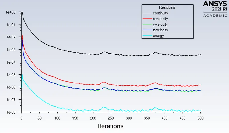
The solution is run for around 500 iterations, and the convergence plot of the residual monitors and processor average temperature during the solution is shown below:
| Residual Monitor | Processor Temperature |
 |
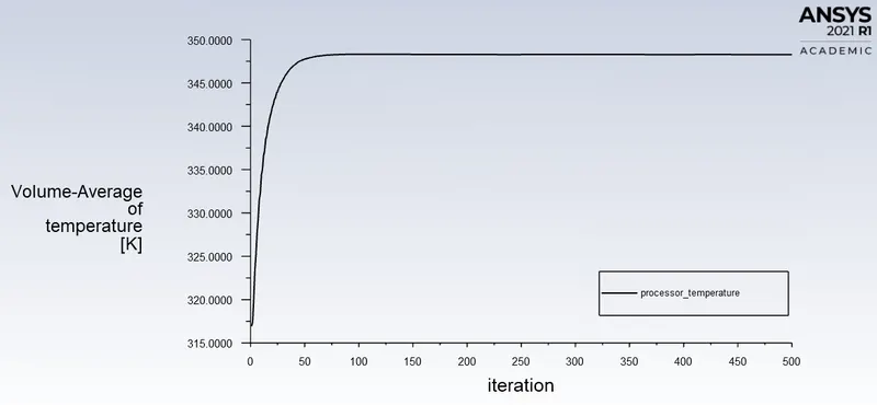 |
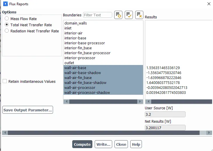
From the above plots, it can be seen that the solution residuals have a repetitive pattern and the processor average temperature reaches a steady-state value after 200 iterations. Hence the solution converges after 200 iterations. Also, the below heat flux report confirms that the applied 3.2 W heat to the processor is dissipated to the surrounding air and other components. Hence solution has converged.
Total Heat balance:
Refined Mesh:
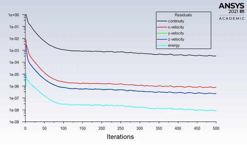
The solution is run for around 500 iterations, and the convergence plot of the residual monitors and processor average temperature during the solution is shown below:
| Residual Monitor | Processor Temperature |
 |
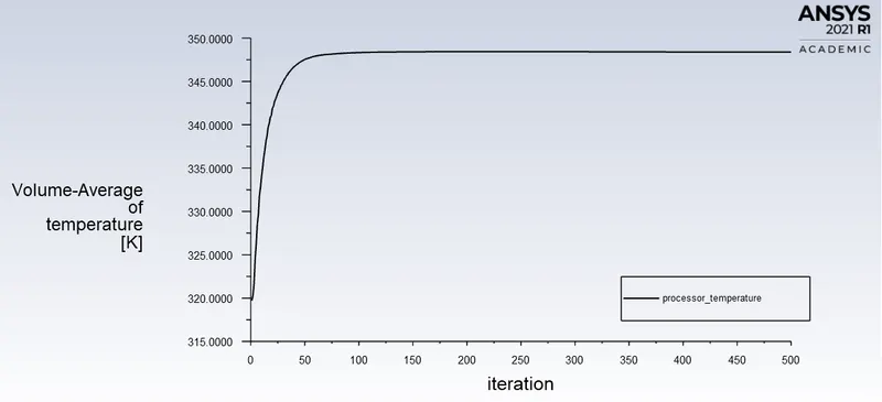 |
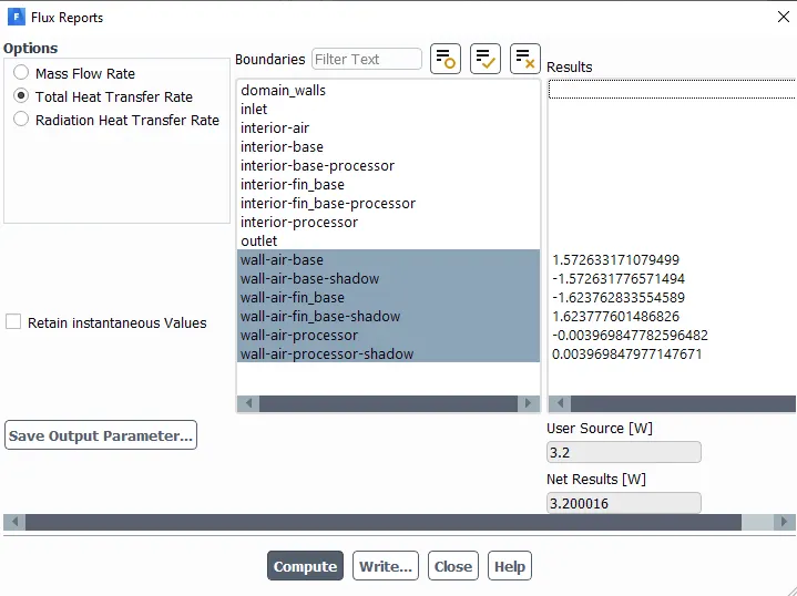
From the above plots, it can be seen that the solution residuals have fallen below desired range after 350 iterations and the processor average temperature reaches a steady-state value after 300 iterations. Hence the solution converges after 350 iterations. Also, the below heat flux report confirms that the applied 3.2 W heat to the processor is dissipated to the surrounding air and other components. Hence solution has converged.
Total Heat balance:
Comparison of the Results:
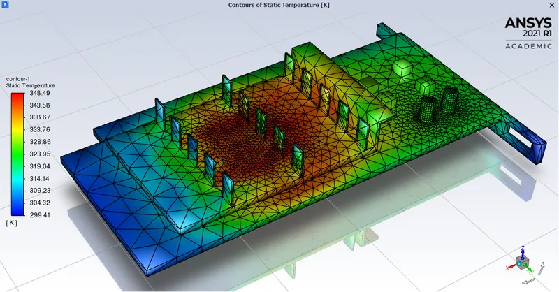
| Coarse Mesh- Temperature distribution in the graphics card | Refined Mesh - Temperature distribution in the graphics card |
 |
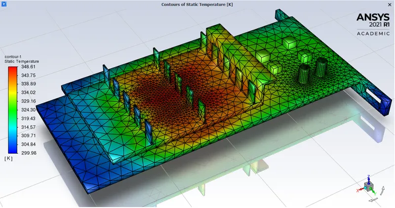 |
The above plots represent the steady-state temperature attained by the processor when the air of velocity 1.5 m/sec flows over it for the coarse and refined mesh cases. It can be seen that the heat is more diffused in the refined mesh case when compared to the coarse mesh. Also, the gradients of temperature are more uniformly distributed in the refined mesh case resulting in fewer hotspots other than the processor-fin area. But, in coarse mesh case, the gradients are not evenly distributed and hotspots are present at the processor-fin area as well as other regions of the fin structure. The following table gives more details about the effect of mesh on the temperature distribution in the graphics card.
| Property | Coarse mesh | Refined mesh |
| Max-Temperature in graphics card | 348.49 K | 348.61 K |
| Temperature gradients in the cells | Non-uniform | Slightly more uniform than coarse mesh case |
| Hotspots | Processor-fin area and other regions (see temperature contour above) | Processor-fin area and other regions, but fewer than coarse mesh case (see temperature contour above) |
| Ratio of difference in heat generated to heat dissipated to heat generated | 0.00365% | 0.0005% |
From the above table, it can be observed that the maximum temperature attained in the refined mesh case is slightly lesser than the coarse mesh case. Hence, the mesh size (quality) has an effect on heat dissipation. Also, the Ratio of difference in heat generated to heat dissipated to that of heat generated in refined mesh case is lesser than that of coarse mesh case. This indicates better heat dissipation is achieved with mesh refinement. Although the improvement in heat dissipation is very small, further refinement of mesh density near the processor-fin, the processor-base regions will significantly affect the results. But due to ANSYS Fluent academic version cell count limitation, further refinement could not be achieved. Hence the refined mesh size mentioned above is used for the following 2.5 and 4.5 m/sec coolant air velocity cases.
Case 2: Refined mesh with Air velocity 2.5 m/sec
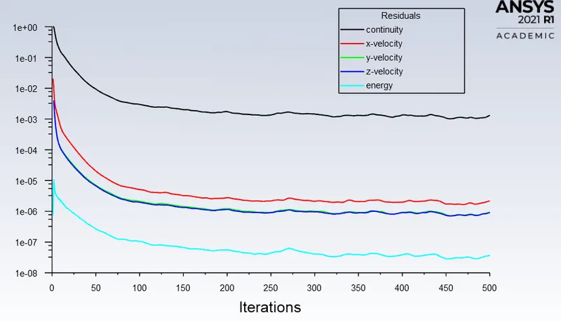
The solution is run for around 500 iterations, and the convergence plot of the residual monitors and processor average temperature during the solution is shown below:
| Residual Monitor | Processor Temperature |
 |
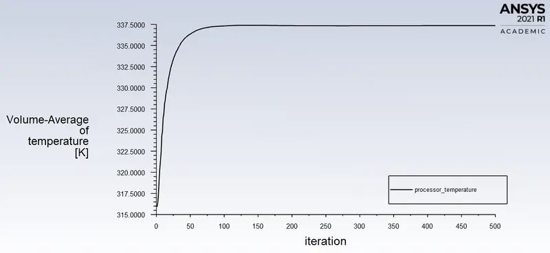 |
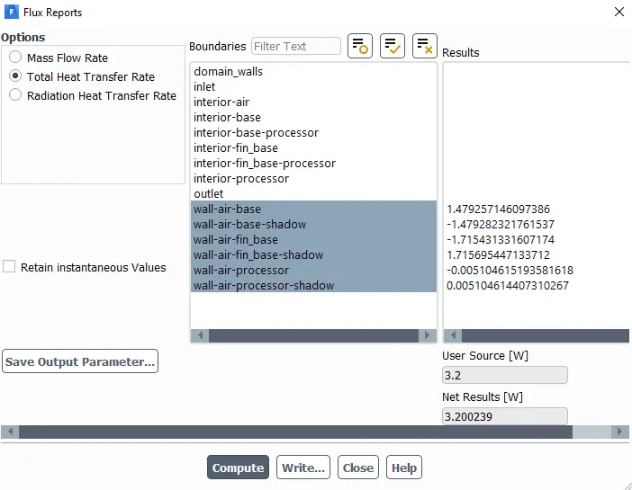
From the above plots, it can be seen that the solution residuals have fallen below desired after 400 iterations and the processor average temperature reaches a steady-state value after 300 iterations. Hence the solution converges after 450 iterations. Also, the below heat flux report confirms that the applied 3.2 W heat to the processor is dissipated to the surrounding air and other components. Hence solution has converged.
Total Heat balance:
Case 3: Refined mesh with Air velocity 4.5 m/sec
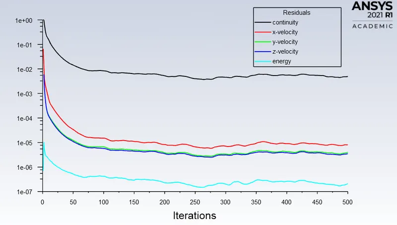
The solution is run for around 500 iterations, and the convergence plot of the residual monitors and processor average temperature during the solution is shown below:
| Residual Monitor | Processor Temperature |
 |
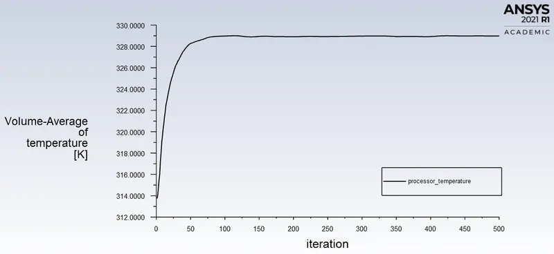 |
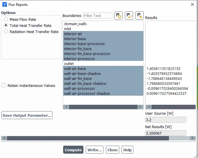
From the above plots, it can be seen that the solution residuals have fallen below desired after 350 iterations and the processor average temperature reaches a steady-state value after 300 iterations. Hence the solution converges after 350 iterations. Also, the below heat flux report confirms that the applied 3.2 W heat to the processor is dissipated to the surrounding air and other components. Hence solution has converged.
Total Heat balance:
| Temperature distribution (Air Velocity - 2.5 m/sec) | Temperature distribution (Air Velocity - 4.5 m/sec) |
 |
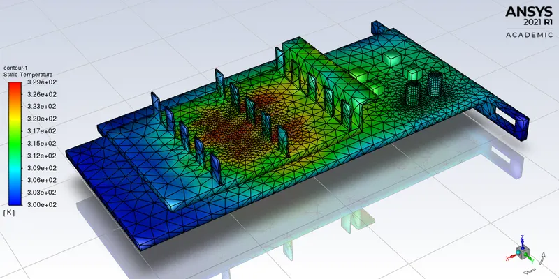 |
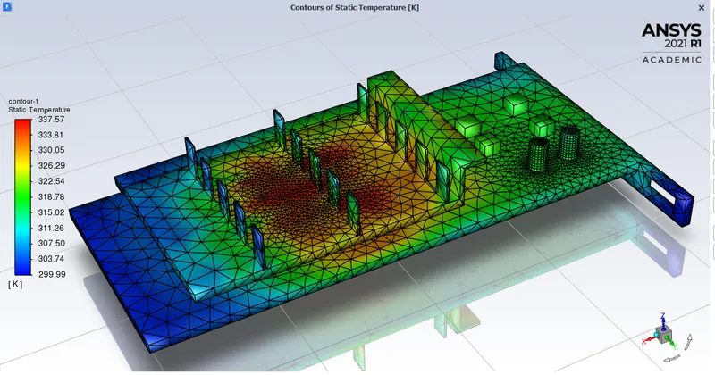
It can be seen from the above figures that, max temperature attained by the graphics card is lesser when the coolant fluid velocity increases. Also, the hotspots are more concentrated near the processor-fin region surroundings in the higher coolant velocity case when compared to the lesser coolant velocity case where the hotspots are distributed throughout the fin part.
The following table gives a broader picture of the effect of coolant velocity and mesh size on heat dissipation and temperature distribution in the graphics card.
| Parameter | Coarse mesh | Refined mesh - Case2 | Refined mesh - Case3 | Refined mesh - Case4 |
| Max Temperature attained by the graphics card processor | 348.490 K | 348.253 K | 337.213 K | 329.186 K |
| Average Surface heat transfer coefficient attained by the graphics card processor | 2.056 w/m^2-K | 2.066 w/m^2-K | 3.25 w/m^2-K | 7.490 w/m^2-K |
From the above table, it can be inferred that mesh quality has an effect on heat dissipation and hotspot generation. Refining the mesh and improving its quality will improve the heat dissipation characteristics. The maximum heat temperature attained by the processor reduces as the coolant velocity increases. The heat transfer coefficient also increases as the coolant velocity is increased resulting in better heat removal from the graphics card components. Hence, choosing an optimum refined mesh with good element quality along with an optimum forced convection model of cooling fluid can improve the heat dissipation from the graphics card. Further, the construction and thermal material properties of the heat-sink (fins) also improves the heat dissipation characteristics.
Conclusion:
Conjugate heat transfer (CHT) analysis of a typical graphics card is carried out in this project with air as the cooling fluid. The main objective is to study the CHT around a graphics card dissipating heat. The CFD model mesh quality and size effects the heat distribution, temperature gradients, and presence of hot spots in the graphics card. The main hot spot is near the processor-heat sink (fin) area along with areas where mesh quality was not good. Optimum forced convection model (fluid side) along with better design (thermal and geometric properties) of the heat sink (solid side) can improve the conjugate heat transfer characteristics of the graphics card, resulting in maintaining the graphics card at operating temperatures. This enhances the computing performance and life of the graphics card.