Calculate the Stretch Ratio by comparing the ELFORM (-2,-1,1,2) with Ogden_Material Model.
Aim:
To Create a block of 10 mm x 10 mm x 10 mm dimension with 10 elements for each direction and use the Ogden_Material card given and simulate the model for Tensile behaviour using different ELFORM 1, -1, 2, -2 and to compare the results.
Deck Setup:
1. Creating Solid Mesh:
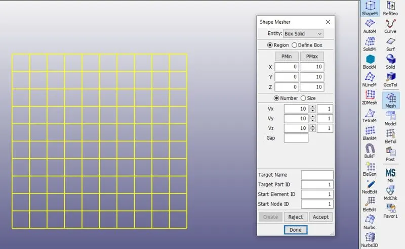
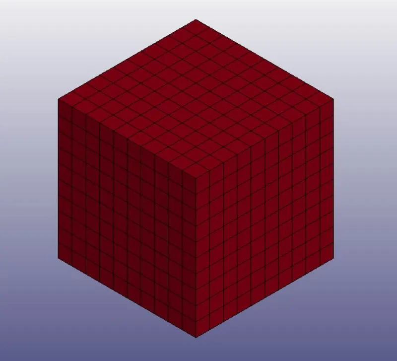
To Create a block of 10mmx10mmx10mm dimension with 10 elements go to Mesh - Shape Mesher and enter the required dimensions as shown.
2. Section Card:
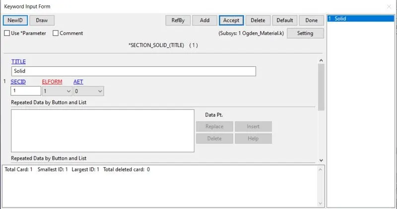
SECTION_SOLID is used and ELFORM is kept as 1 for first simulation and is changed for other simulations ELFORM -1, 2 & -2.
3. Part Card:
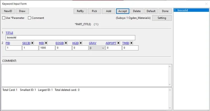
The Created Section ID and the provided Material ID are assigned to the created part.
4. Creating Boundry Conditions:
Go to Create entity and create 3 sets of Boundary SPC as shown to fix one face as shown.
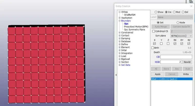
Constraining the nodes in X DOF
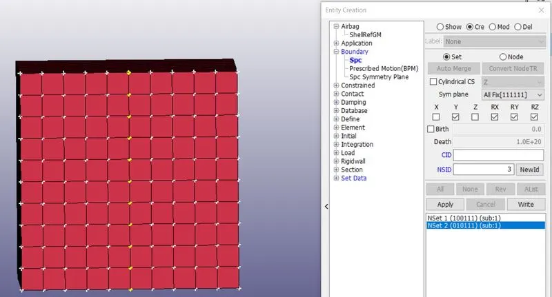
Constraining the Middle nodes in Y DOF along Z axis
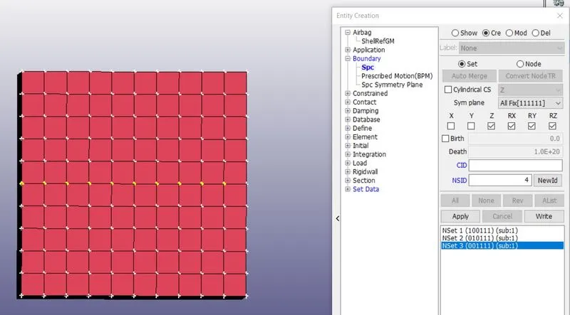
Constraining the Middle nodes in Z DOF along Y Axis
The Nodes fixed on a single face is fixed and is restricted to move along the x axis as well as the rotational DOF is arrested.
The Nodes on the middle are fixed to the respective DOF.
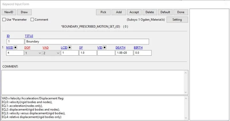
5. Boundary Prescribed Motion:
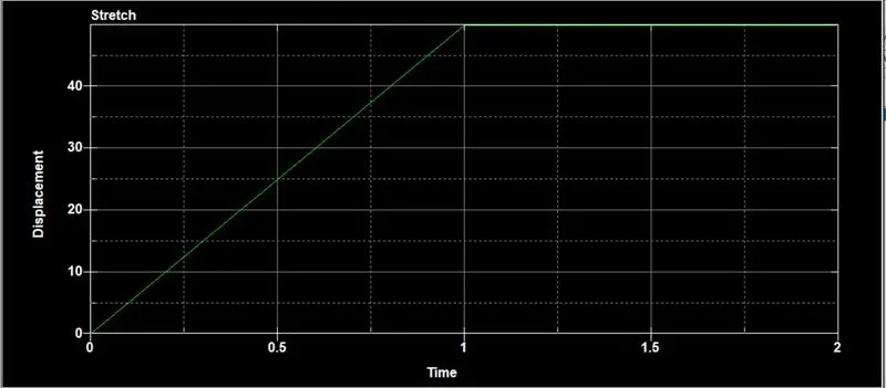
Before setting up the BOUNDARY_PRESCRIBED_MOTION_SET the displacement has to be calculated.
Stretch Ratio = `lambda = 1 + epsi_e`
`epsi_e`= Engineering Strain = `(dell)/l`
`5 = 1 + ((dell)/10)`
`dell = 40 mm`
From the above the displacement curve is defined with 50 mm as shown.
6. Control Cards:
Implicit control cards are setup as shown below.
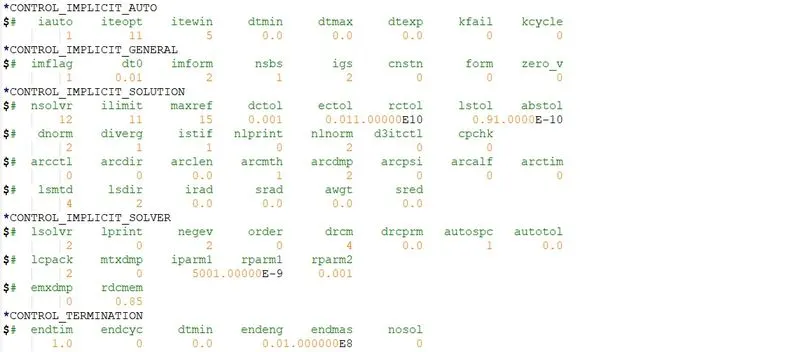
> In CONTROL_IMPLICIT_GENERAL imflag is set as 1 to run the simulation in Implicit.
> The CONTROL_IMPLICIT_AUTO adjusts the time step for convergence within the iteopt and itewin values.
> The CONTROL_IMPLICIT_SOLUTION card is used to specify whether a linear or nonlinear solution is desired.
> The CONTROL_IMPLICIT_SOLVER card is used to apply implicit calculations. The linear equation solver performs the CPU-intensive stiffness matrix inversion.
> CONTROL_TERMINATION is used to define the end time.
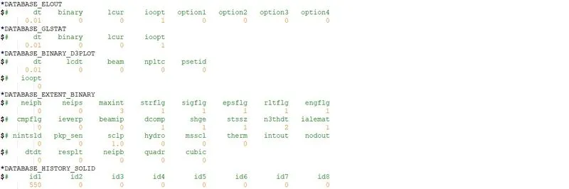
7. Output Cards:
Output card are defined to display the output given by the solver after running the simulation.
Output:
ELFORM 1
X Stress
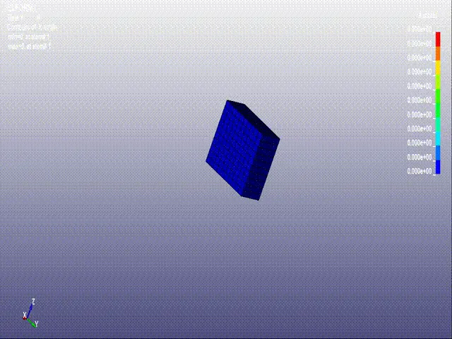
X Strain
ELFORM -1
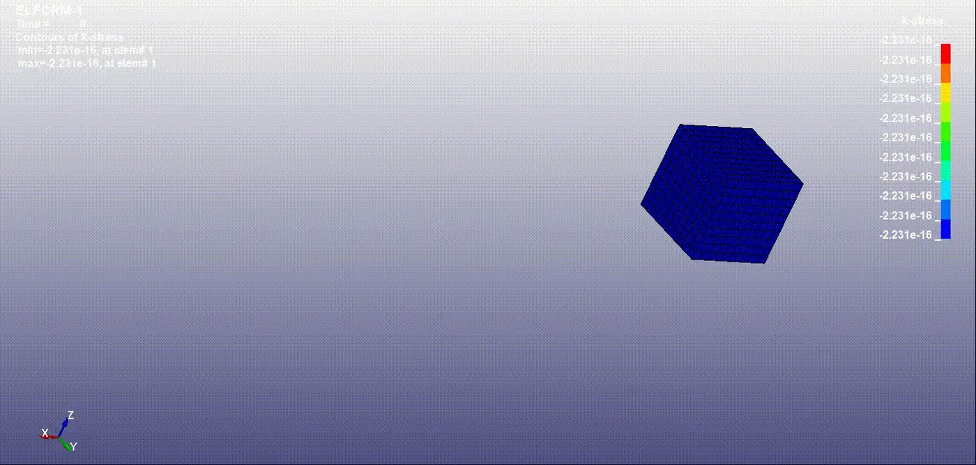
X Stress
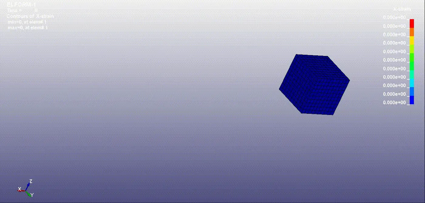
X Strain
ELFORM 2
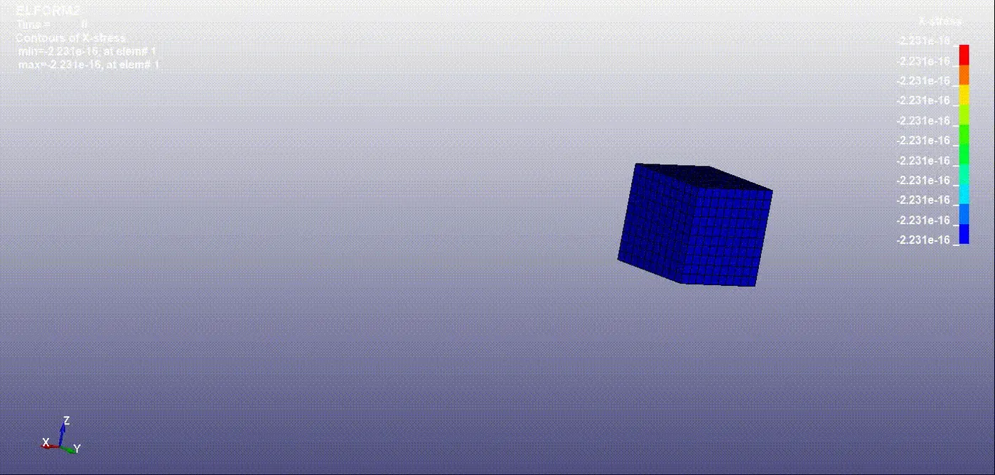
X Stress
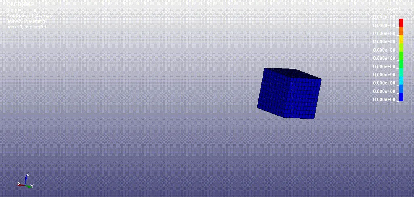
X Strain
ELFORM -2
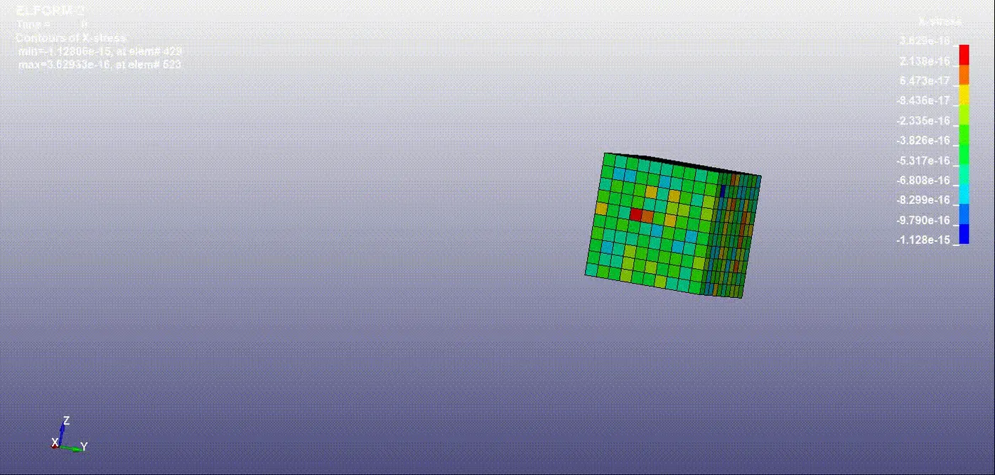
X Stress
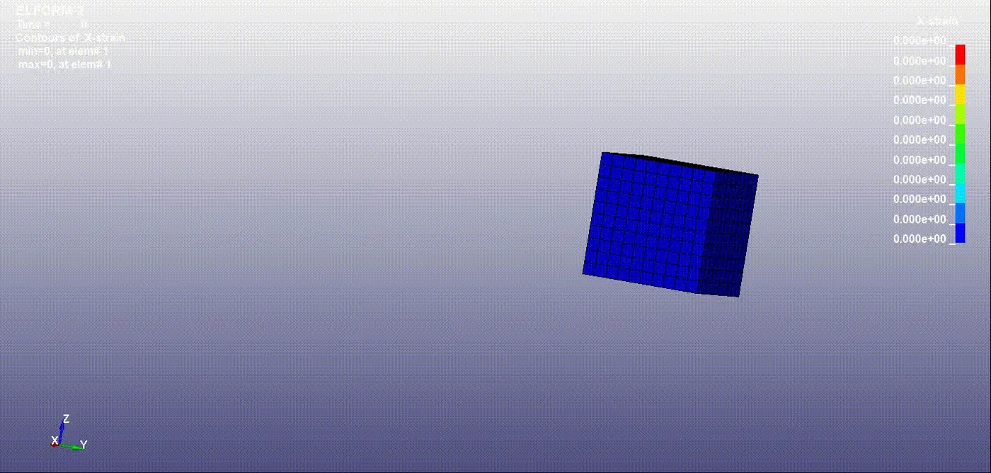
X Strain
The Stress and Strain for an element is saved from selecting the element and plotting the X Stress and X Strain as shown.
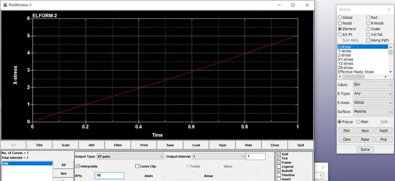
The Stress and Strain values obtained are True Stress and True Strain. The Engineering Stress and Engineering strain are calculated as follows.
True Stress `sigma_t = sigma_e(1 + epsi_e)`
Engineering Stress `sigma_e = (sigma_t/(1 + epsi_e))`
True Strain `epsi_t = ln (1 + epsi_e)`
Engineering Strain `epsi_e = e^(epsi_t) - 1`
Stretch Ratio `lambda = 1 + epsi_e`
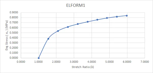
| ELFORM 1 | |||||
| Time (ms) | True Values | Engineering Values | Stretch Ratio | ||
| X-Strain | X-Stress (Mpa) | X-Strain | X-Stress (Mpa) | ||
| 0.00 | 0.0000 | 0.0000 | 0.0000 | 0.0000 | 1.0000 |
| 0.11 | 0.4369 | 0.5942 | 0.5479 | 0.3839 | 1.5479 |
| 0.22 | 0.7388 | 1.1225 | 1.0934 | 0.5362 | 2.0934 |
| 0.33 | 0.9749 | 1.6365 | 1.6509 | 0.6173 | 2.6509 |
| 0.44 | 1.1659 | 2.1584 | 2.2089 | 0.6726 | 3.2089 |
| 0.56 | 1.3257 | 2.7011 | 2.7648 | 0.7175 | 3.7648 |
| 0.67 | 1.4619 | 3.2691 | 3.3142 | 0.7578 | 4.3142 |
| 0.78 | 1.5821 | 3.8547 | 3.8653 | 0.7923 | 4.8653 |
| 0.89 | 1.6892 | 4.4406 | 4.4153 | 0.8200 | 5.4153 |
| 1.00 | 1.7878 | 5.0232 | 4.9760 | 0.8406 | 5.9760 |
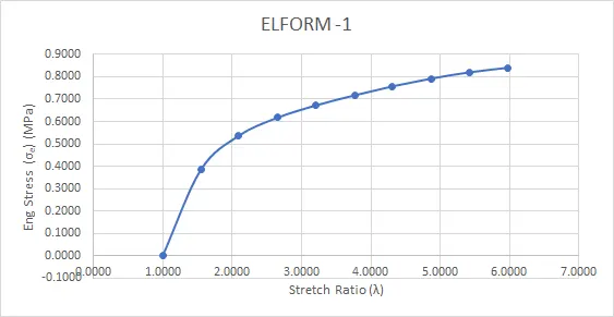
| ELFORM -1 | |||||
| Time (ms) | True Values | Engineering Values | Stretch Ratio | ||
| X-Strain | X-Stress (Mpa) | X-Strain | X-Stress (Mpa) | ||
| 0.00 | 0.0000 | 0.0000 | 0.0000 | 0.0000 | 1.0000 |
| 0.11 | 0.4369 | 0.5942 | 0.5479 | 0.3839 | 1.5479 |
| 0.22 | 0.7389 | 1.1228 | 1.0937 | 0.5363 | 2.0937 |
| 0.33 | 0.9750 | 1.6368 | 1.6513 | 0.6173 | 2.6513 |
| 0.44 | 1.1656 | 2.1576 | 2.2080 | 0.6726 | 3.2080 |
| 0.56 | 1.3255 | 2.7004 | 2.7641 | 0.7174 | 3.7641 |
| 0.67 | 1.4618 | 3.2689 | 3.3138 | 0.7578 | 4.3138 |
| 0.78 | 1.5823 | 3.8552 | 3.8663 | 0.7922 | 4.8663 |
| 0.89 | 1.6898 | 4.4433 | 4.4184 | 0.8200 | 5.4184 |
| 1.00 | 1.7877 | 5.0228 | 4.9755 | 0.8406 | 5.9755 |
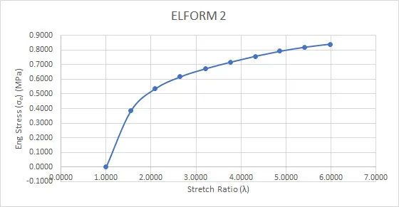
| ELFORM 2 | |||||
| Time (ms) | True Values | Engineering Values | Stretch Ratio | ||
| X-Strain | X-Stress (Mpa) | X-Strain | X-Stress (Mpa) | ||
| 0.00 | 0.0000 | 0.0000 | 0.0000 | 0.0000 | 1.0000 |
| 0.11 | 0.4369 | 0.5942 | 0.5479 | 0.3839 | 1.5479 |
| 0.22 | 0.7389 | 1.1228 | 1.0937 | 0.5363 | 2.0937 |
| 0.33 | 0.9749 | 1.6365 | 1.6510 | 0.6173 | 2.6510 |
| 0.44 | 1.1656 | 2.1572 | 2.2079 | 0.6725 | 3.2079 |
| 0.56 | 1.3255 | 2.7002 | 2.7639 | 0.7174 | 3.7639 |
| 0.67 | 1.4619 | 3.2689 | 3.3141 | 0.7577 | 4.3141 |
| 0.78 | 1.5822 | 3.8545 | 3.8657 | 0.7922 | 4.8657 |
| 0.89 | 1.6898 | 4.4432 | 4.4184 | 0.8200 | 5.4184 |
| 1.00 | 1.7877 | 5.0223 | 4.9755 | 0.8405 | 5.9755 |
| ELFORM -2 | |||||
| Time (ms) | True Values | Engineering Values | Stretch Ratio | ||
| X-Strain | X-Stress (Mpa) | X-Strain | X-Stress (Mpa) | ||
| 0.00 | 0.0000 | 0.0000 | 0.0000 | 0.0000 | 1.0000 |
| 0.11 | 0.4369 | 0.5942 | 0.5479 | 0.3839 | 1.5479 |
| 0.22 | 0.7389 | 1.1228 | 1.0937 | 0.5363 | 2.0937 |
| 0.33 | 0.9749 | 1.6365 | 1.6510 | 0.6173 | 2.6510 |
| 0.44 | 1.1656 | 2.1572 | 2.2079 | 0.6725 | 3.2079 |
| 0.56 | 1.3255 | 2.7002 | 2.7639 | 0.7174 | 3.7639 |
| 0.67 | 1.4619 | 3.2689 | 3.3141 | 0.7577 | 4.3141 |
| 0.78 | 1.5822 | 3.8545 | 3.8657 | 0.7922 | 4.8657 |
| 0.89 | 1.6898 | 4.4432 | 4.4184 | 0.8200 | 5.4184 |
| 1.00 | 1.7877 | 5.0223 | 4.9755 | 0.8405 | 5.9755 |
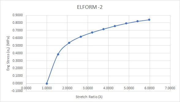
From the above graphs the engineering stress value is around 0.85 MPa for the stretch ratio of 5 where as for the given graph the the Stress value is around 1.6 MPa.
Explicit Analysis:
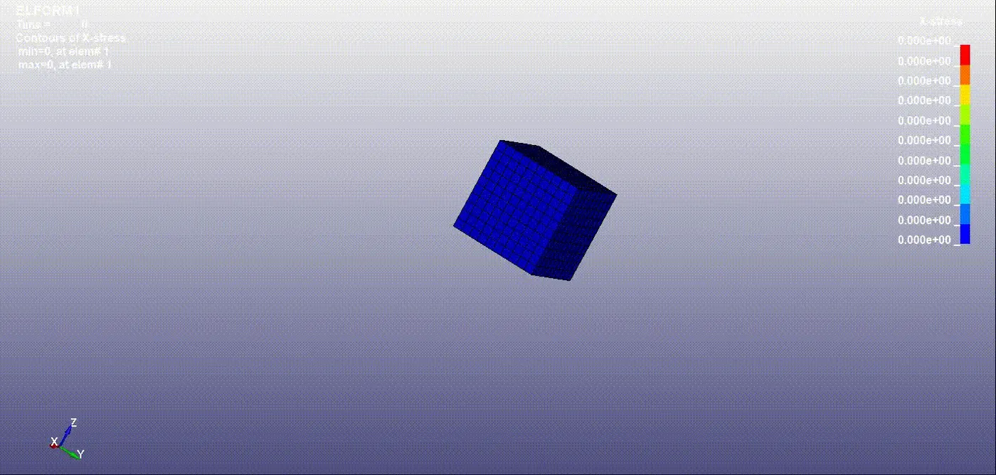
The Same deck is used for explicit analysis without using the implicit control cards and the simulation is run and the following output is obtained.
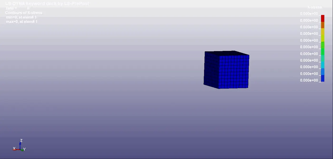
The above failure of the elements is due to the residual forces where the convergence is not obtained in explicit method.
Conclusion:
From the above explicit method method is not suitable for running analysis on this model as it is not able to obtain the convergence due to which the residual forces are overlapping. Implicit analysis provides better results for solving the problems which are time dependent.