Week-6 Calculate the Stretch Ratio by comparing the ELFORM (-2,-1,1,2) with Ogden_Material Model.

Aim: To simulate tensile behavior of a 10mm cube using Ogden material properties, apply boundary conditions, and compare results with a given uniaxial plot up to a stretch ratio of 5. Evaluate different element formulations (ELFORM = 1, 2, -1, -2) and adjust material units. Choose and justify the use of an implicit or explicit solver.

Introduction: The Ogden material model, created by Raymond Ogden in 1972, describes the non-linear stress-strain behavior of complex materials like rubber, polymers, and biological tissues. It uses a strain energy density function to derive stress-strain relationships, making it ideal for modeling rubbery and biological materials at higher strains.

Explanation: Since the simulation is very slow (quasi-static), we can ignore inertial effects and use implicit analysis. Hyperelastic materials require steps and iterations to reach equilibrium, even with implicit analysis.

Element formulations used are ELFORM 1, -1, 2, and -2 for solids:

• ELFORM 1: Under-integrated constant stress; needs hourglass stabilization; efficient and accurate.
• ELFORM 2: Reduced integrated; no hourglass stabilization needed; slower than ELFORM 1; shear locking can occur.
• ELFORM -1: Similar to ELFORM 2 but accounts for shear locking; efficient (CPU time).
• ELFORM -2: Similar to ELFORM -1 but more accurate; higher computational cost.
  

Deliverables:

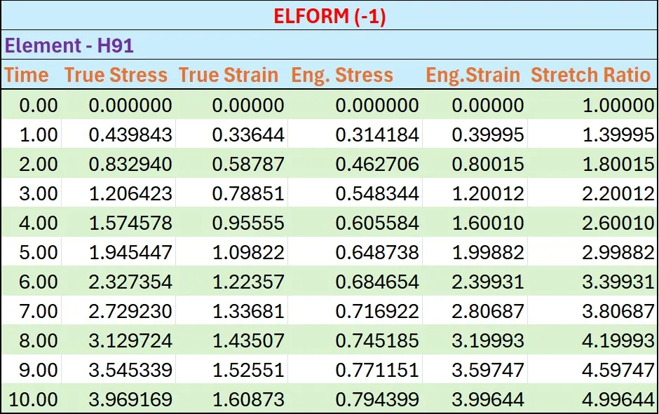
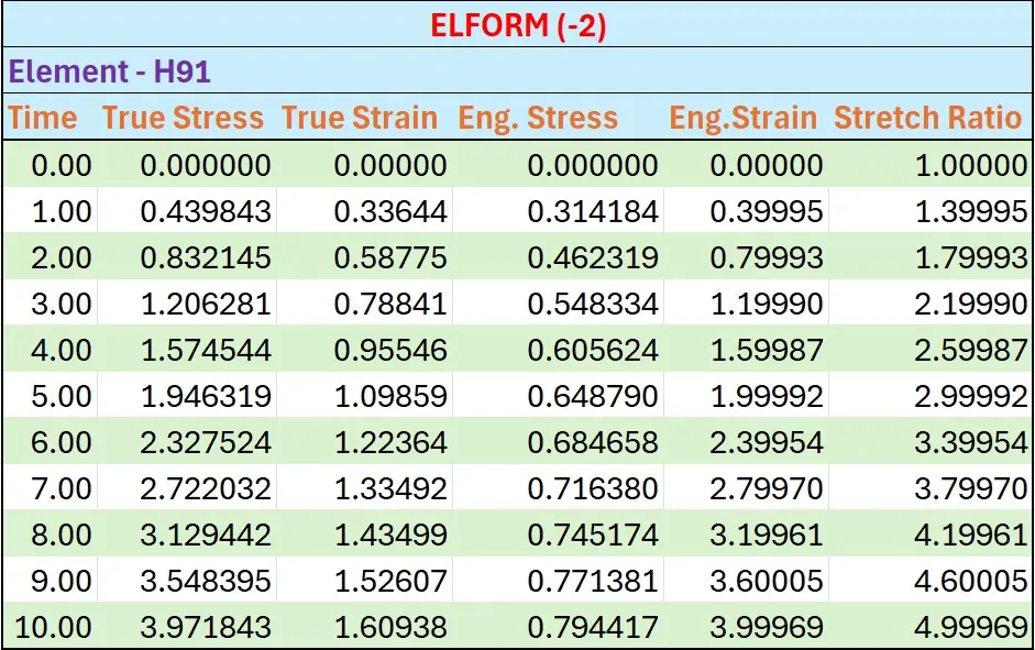
• An excel sheet with proper conversion and calculation of stress/Strain Ratio for all the ELFORM.
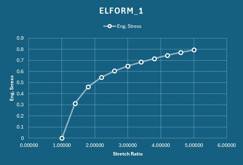
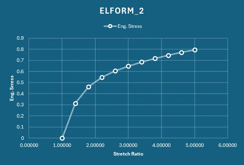
• A proper image of the plot comparison of various ELFORMS against the Uniaxial Plot Given in the challenge.

Procedure:

1. Open LS Dyna and Open the given model file.

2. Create the cube of size 10mm x 10 mm x 10 mm.

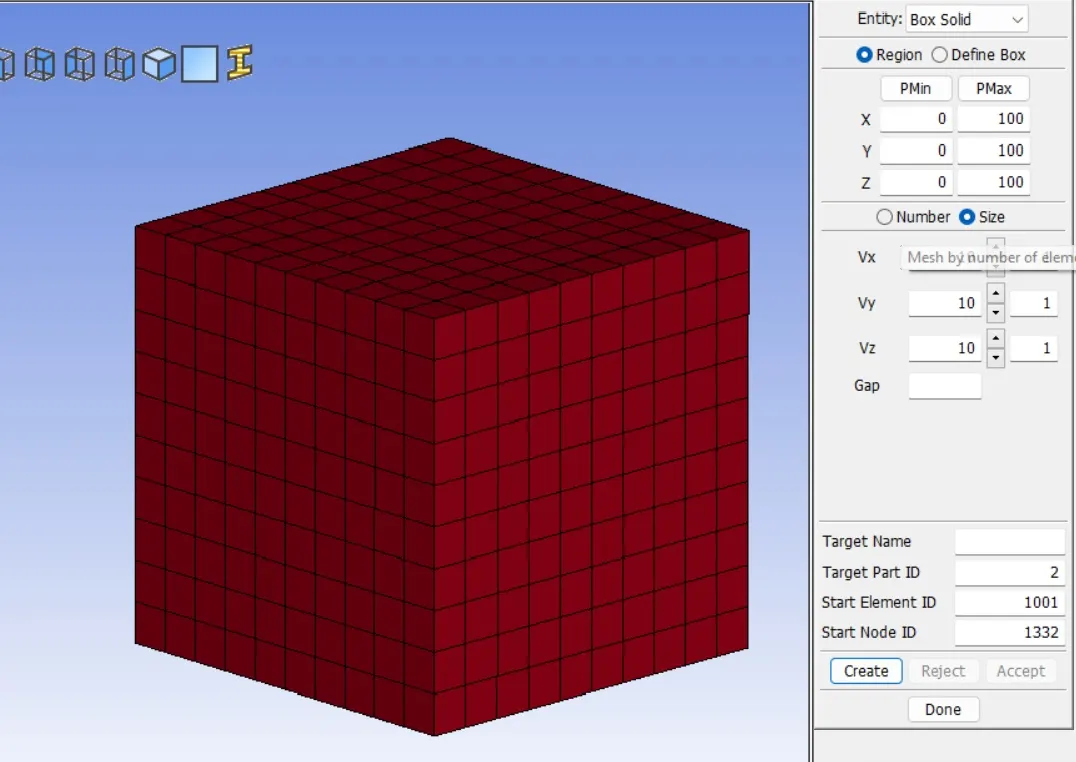
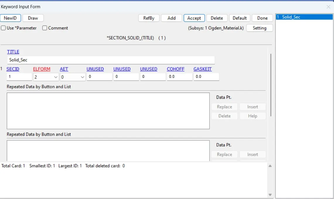
3. Create the section Card.

For this go to Model and Part > Keyword > all > section > solid > Title = "Solid_Sec" > ELFORM = 2

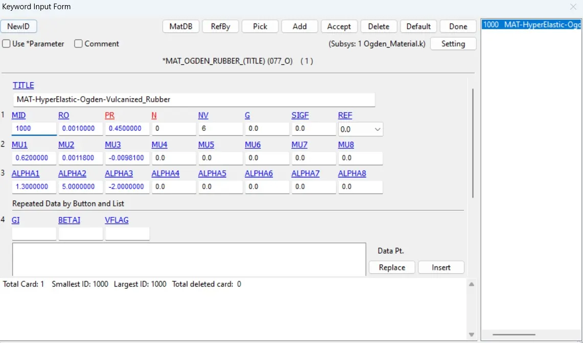
4. Material Card is created already in the given model.

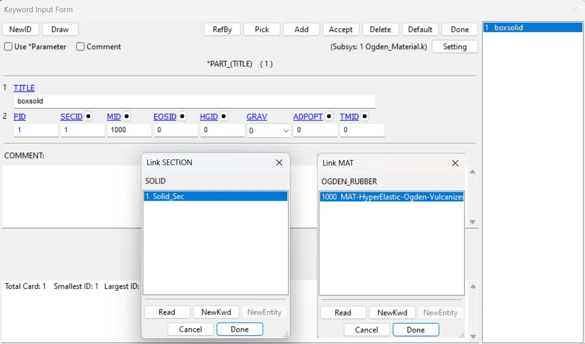
5. Assign Material Card and Section Card to Part.

6. Boundary Condition:

6A. Fix the Bottom of Cube

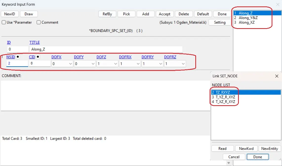
To fix the Bottom face, we will use different set of nodes and using single point constraint boundary, we can allow or constraint the nodes with different degrees of freedom.

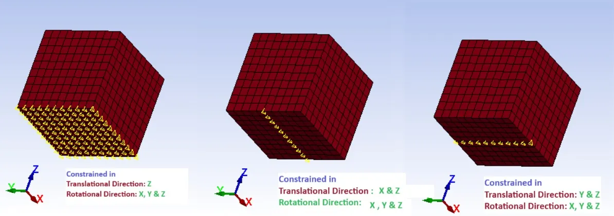
As shown in above image, constraints are given for the different set of nodes in a way that cube can shrink in X and Y direction upon tension in Z-Direction and also stick to its position.

Thus , this boundary condition can be relatable to the real-time boundary condition.

6B. Apply Prescribed Motion to top Surface

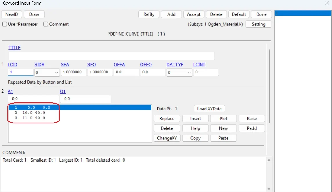
1. First Define the Load Curve

Since Stretch Ratio is 5.

And Stretch ratio = 1 + engineering strain

5 = 1+(Displacement / Original length )

5 = 1 + (Displacement / 10 )

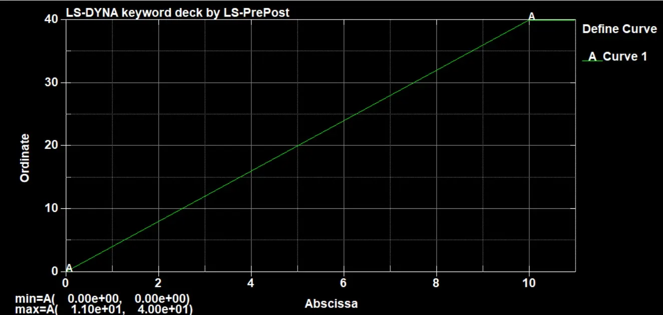
Displacement = 40 mm

Final Length = 50 mm

So the face is to be displaced by a minimum of 40mm.

go to Model and Part > Keyword > All > Define > Curve > As follows

2. Now Create Top Surface Node Set

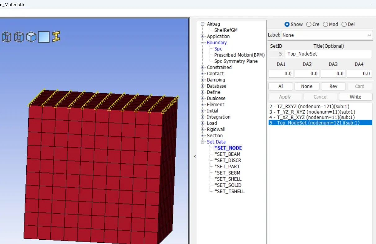
3. Now go to create the prescribed boundary condition by the following steps.

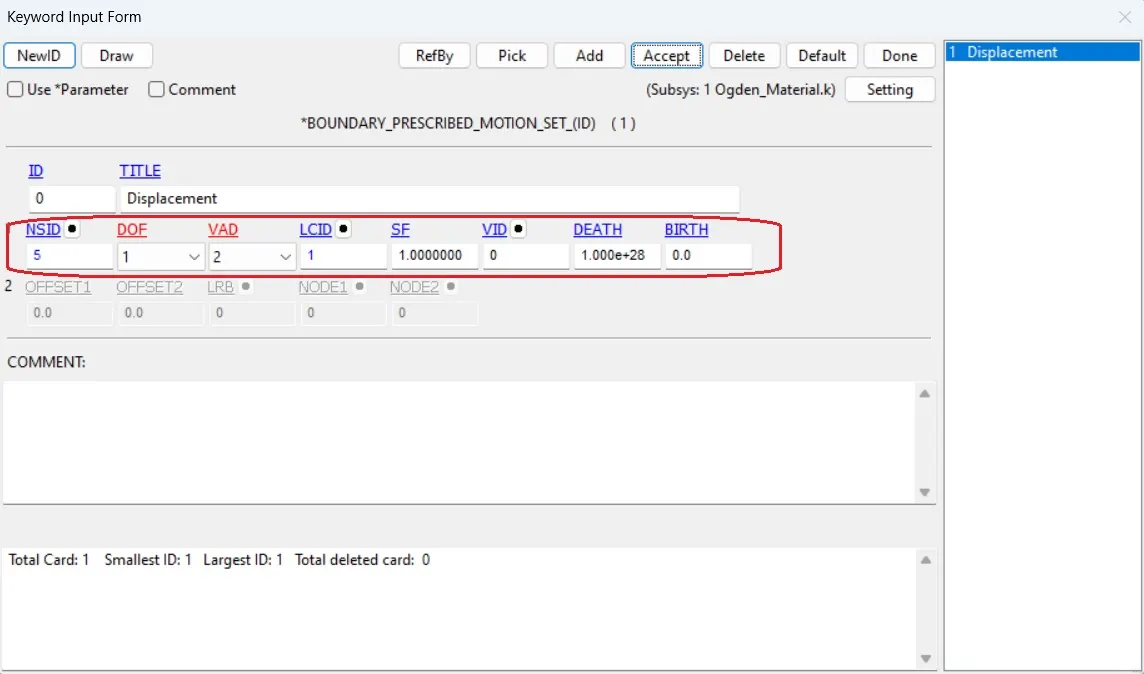
model > keyword manager > all > prescribed motion set id > assigned the created displacement nodeset id > assigned the created displacement curve > accept and done.

7. Control Cards

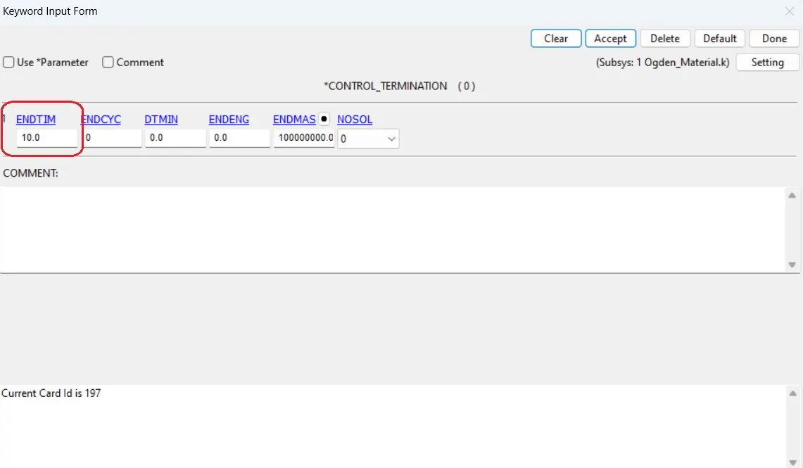
1. CONTROL TERMINATION CARD

The main purpose of control termination card is to stop the job.

Go to model and part > keyword manager > control > termination > specify termination time is 10 ms > accept and done.

2. CONTROL IMPLICIT CARDS

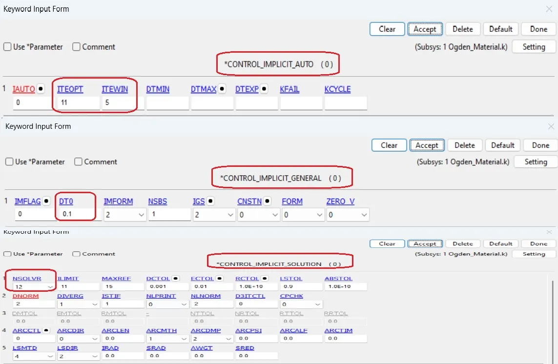
It is nonlinear implicit analysis we need to create implicit cards like implicit auto, implicit general and implicit solution and control termination for the model.

For this go to model and part > keyword manager > control > IMPLICIT_AUTO > specified the required values > accept and done.

Similalry Specify the IMPLICIT_GENERAL & IMPLICIT_SOLUTION

8. DATABASE CARDS

To extract the results we need to create a database cards for the model.

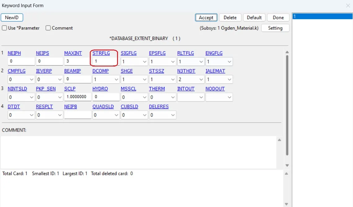
EXTEND_BINARY

To generate the strain outputs go to model > keyword manager > all > DATABASE > EXTEND_BINARY> and give STRFLG as ‘1’, this is due to extract the true strain values for the model and accept the card.

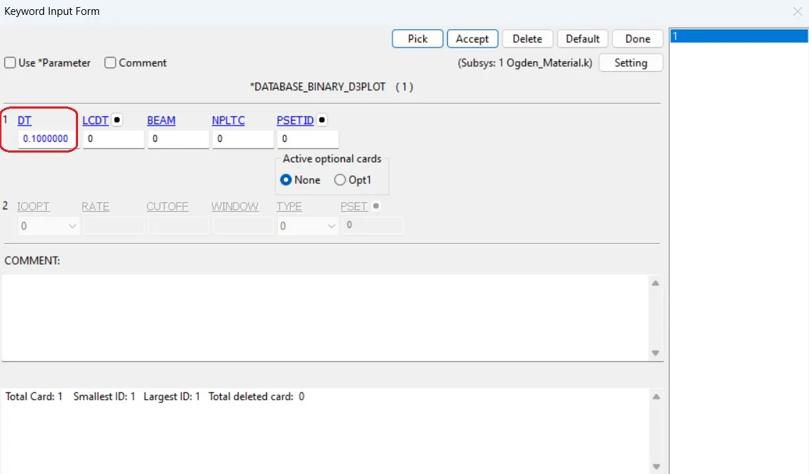
OUTPUT DATABASE AS BINARY D3 PLOT

Go to model and part > keyword manager > database > select DATABASE_BINARY_D3PLOT > provide DT value is 0.1 is a time interval between output states > accept & done.

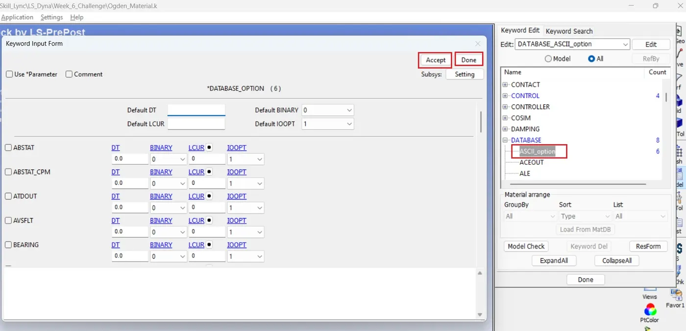
OUTPUT DATABASE AS ASCII

model and part > keyword manager > database > select ASCII_option > check GLSTAT,MATSUM ,NODOUT, SECFORC, SLEOUT, RCFORCE > specify all value is 0.1>accept & done

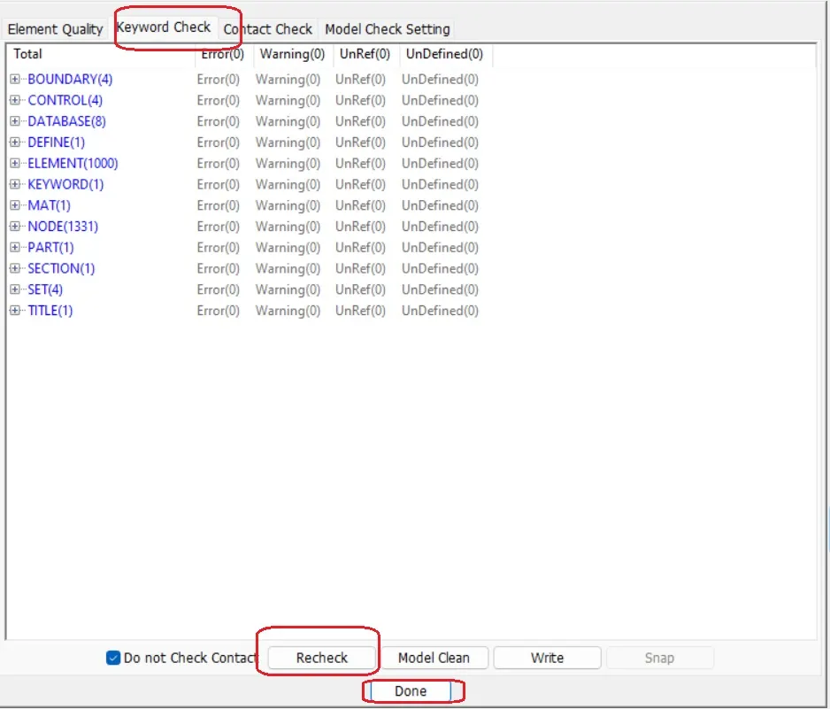
9. MODEL CHECKUP AND RUN THE SIMULATION

10. Run the Simulation

Save the file for different ELFORM i.e, 1, -1, 2, -2
Run the Simulation in LS Run and Open for the result analysis in LS Pre-post.

11. Analysis

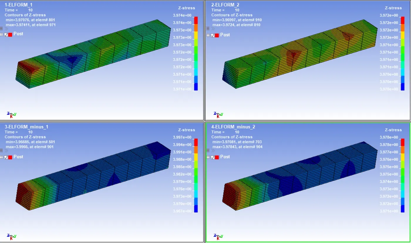
Stress Counter in Z - Direction

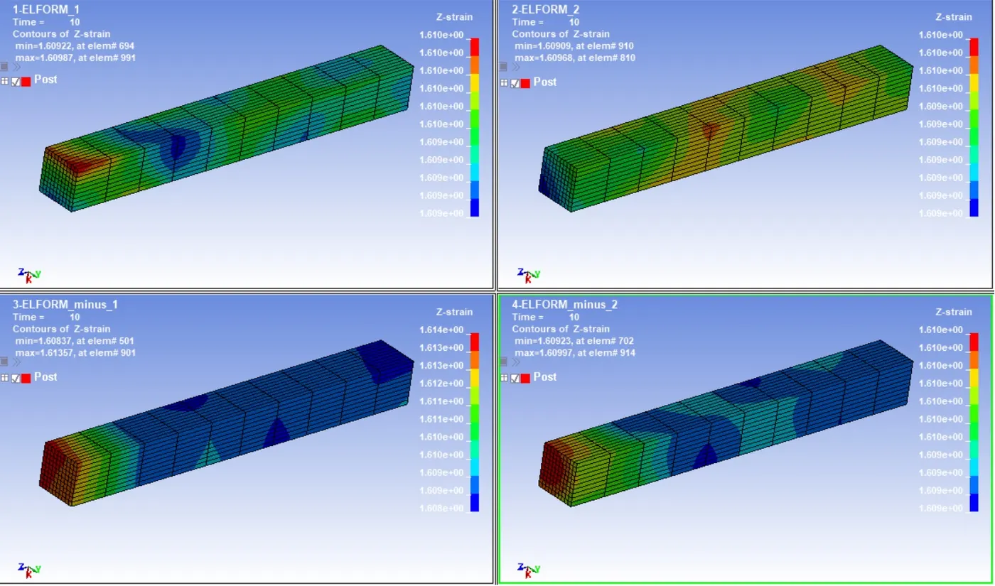
Strain Counter in Z - Direction

Calculation of Nominal Stress and Stretch Ratio

We know that,

Eng. Stress = True Stress /(1 + Eng. Stress)

or, σe= σt/(1+εe)

Eng. Strain = e^(True Strain) - 1

or, εt= e^εt -1

Stretch Ratio = 1 + Eng. Strain

or, λ=1+ εt

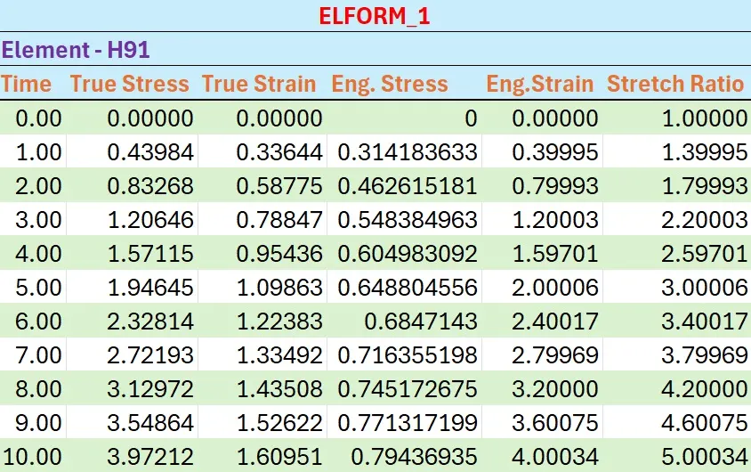
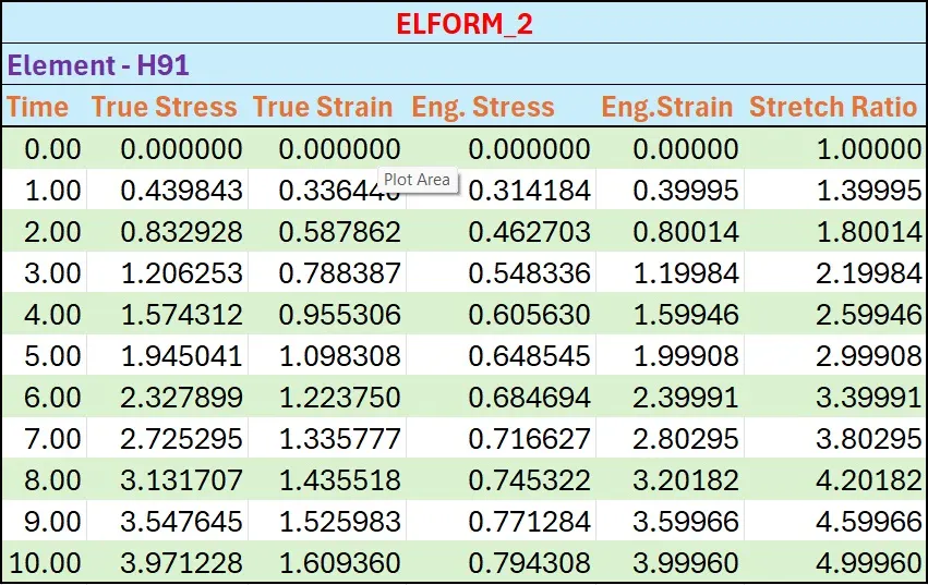
Conversion and calculation of Stress/Strain Ratio for all the ELFORM

ELFORM_1

ELFORM_2

ELFORM (-1)

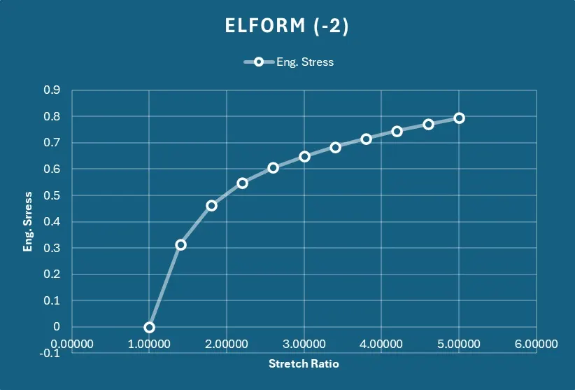
ELFORM (-2)

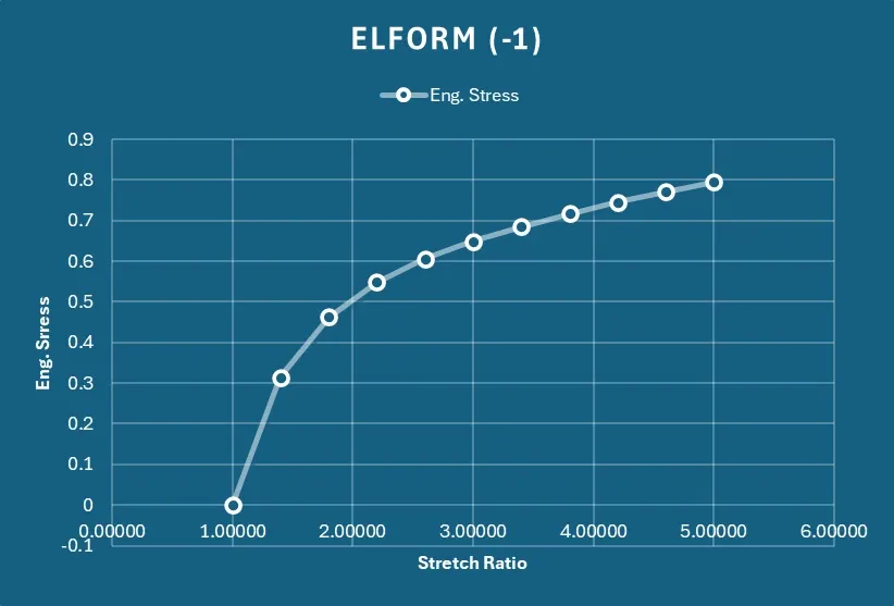
Plot of Eng. Stress Vs Stretch Ratio

ELFORM_1

ELFORM_2

ELFORM (-1)

ELFORM (-2)

Observation

• We can observe the Stress and Strain results are same for different solid element formulations.
• We can observe same stretch ratio for all different element formulations.