Week-6 Calculate the Stretch Ratio by comparing the ELFORM (-2,-1,1,2) with Ogden_Material Model.

Week 6: Calculate the Stretch Ratio by comparing the ELFORM (-2,-1,1,2)

Aim

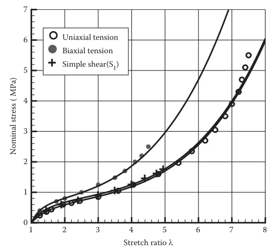
• Create a block of 10mmx10mmx10mm dimension with 10 elements for each direction and use the material card attached (Ogden_Material.k) that is representative of the material properties from the figure below.
  
  
• Use appropriate boundary conditions to simulate the model's tensile behaviour and compare the results from your simulation to the plot above up to stretch ratio 5. Only the uniaxial plot is to be compared.
  
  
• Compare the results for the simulation using ELFORM = 1, 2, -1, -2
  
  
• The unit of µ in the material definition is in MPa and α is a dimensionless quantity. Modify those quantities according to your unit systems.
  
  
• Use a proper solver (Implicit/Explicit) and explain why.
  

Output Required

The following deliveries are needed from the simulation:

• Input file (Keyword File).
  
• Final simulation animation.
  
• An Excel sheet with proper conversion and calculation of Stress/Strain and the Stretch Ratio for all the ELFORM.
  
• A proper image of the plot comparison of various ELFORMS against the Uniaxial Plot is given in the challenge.

Introduction

Ogden_Material

The Ogden material model is a hyperelastic material model used to describe the non-linear stress-strain behaviour of complex materials such as rubbers, polymers, and biological tissues. It was developed by Raymond Ogden in 1972.

Let’s dive into the details:

• The Ogden model assumes that the material behaviour can be described by a strain energy density function. This function relates the strain energy stored in the material to the deformation.
  
• In the Ogden material model, the strain energy density is expressed in terms of the principal stretches (λ₁, λ₂, λ₃):

where 'N,' '𝜇𝑝" role="presentation">μpμpμpμpμpμpμpμpμpμp' and '𝛼𝑝" role="presentation">αpαpαpαpαpαpαpαpαpαp' are material constants.

• The Ogden material model is particularly useful for modelling rubbery and biological materials at high strains.
  
• It provides a more accurate representation of their complex non-linear stress-strain behaviour compared to simpler models like the Neo-Hookean solid.
  

Stretch ratio

The stretch ratio (often denoted as l) aka extension ratio is a fundamental concept in mechanics and materials science. It quantifies the elongation or deformation of a material when subjected to an external force. The stretch ratio is specifically defined as the ratio of the final length to the initial length of the material.

Stretch Ratio = Final Length / Initial Length

l = L_f/L₀

The concept of stretch ratio is utilized in LS-DYNA simulations to analyze engineering stress and strain.

• Engineering Stress and Strain:

We often work with engineering stress and strain in traditional engineering analysis. Engineering stress is calculated as the force applied to a material divided by its original cross-sectional area. It represents the load per unit area.

Engineering strain is the ratio of the change in length (deformation) to the original size of the material.

• True Stress and Strain

However, when dealing with large deformations and nonlinear material behaviour, it’s essential to consider true stress and true strain. True strain accounts for the actual deformation of the material, even when it undergoes significant elongation or compression.

The relationship between engineering strain, true stress and true strain is given by:

Implicit and Explicit Analysis

Implicit and explicit finite element analysis (FEA) are two different approaches used to solve structural problems. Let’s delve into the details:

Implicit Analysis

Implicit analysis, also known as static analysis, involves solving a system of equations that includes both the current and later states of the given system. It is based on the Newton-Raphson method.

For the time incrementation, In implicit analysis, the state of the model is calculated at multiple points in time, and the new state cannot be directly extrapolated from the old state. Instead, a coupled system of equations must be solved.

The applications of implicit analysis include,

1. Steady-State Problems: Implicit analysis is suitable for steady-state problems where the boundary conditions affect the structure slowly.
2. Slowly Changing Loads: When the effects of strain rates are minimal and the increment of stress as a function of strain can be established, implicit methods are preferred.
3. Global Equilibrium: Implicit analysis establishes global equilibrium in the model at each time increment.
   
   

The main advantages are

1. Stable and robust for a wide range of problems.
2. Suitable for linear and nonlinear analyses.
3. Efficient for static and quasi-static problems.
   
   

The main disadvantages are

1. Requires solving a system of equations, making it computationally expensive.
2. Smaller time increments are necessary to maintain stability.
3. May not handle dynamic effects well.

Explicit Analysis

Explicit analysis calculates the state of a system at a different time from the current time. It directly extrapolates the new state from the data available in the current state.

For the time incrementation, explicit analysis uses larger time increments, but stability depends on the material properties and element size. It is commonly used for transient dynamic simulations.

The applications of explicit analysis include,

1. Dynamic Events: Explicit analysis is suitable for dynamic events such as impact, crash, or explosion simulations.
2. High Strain Rates: When strain rates are significant, explicit methods are preferred.
3. Short Duration Phenomena: It excels in capturing short-duration phenomena.
   
   

The main advantages are

1. Efficient for transient dynamic problems.
2. Handles large deformations and nonlinearities.
3. Well-suited for impact and crash simulations.

The main disadvantages are

1. Limited to short-duration events.
2. Requires additional computation due to larger time increments.
3. It can be harder to implement

In summary, implicit analysis is well-suited for problems involving steady-state conditions, where the system achieves equilibrium and remains relatively unchanged over time. Such problems include the structural analysis of buildings under constant loads, heat transfer in steady-state conditions, and the static deformation of mechanical components. Implicit methods are known for their stability and robustness, effectively managing gradual changes.
In situations involving dynamic events or transient phenomena, characterized by swift changes within the system over time, explicit analysis is typically more suitable. Dynamic issues such as car crash simulations, impact analysis, and explosion dynamics are prime examples. Explicit methods are adept at managing events of short duration and are particularly effective for scenarios involving large deformations and high strain rates.

For hyperelastic materials such as the Ogden model, deformations are typically small. Therefore, in this case, to achieve accurate and reliable results, the implicit method is utilized.

Procedure

Step 01: Importing And Inspecting The Model

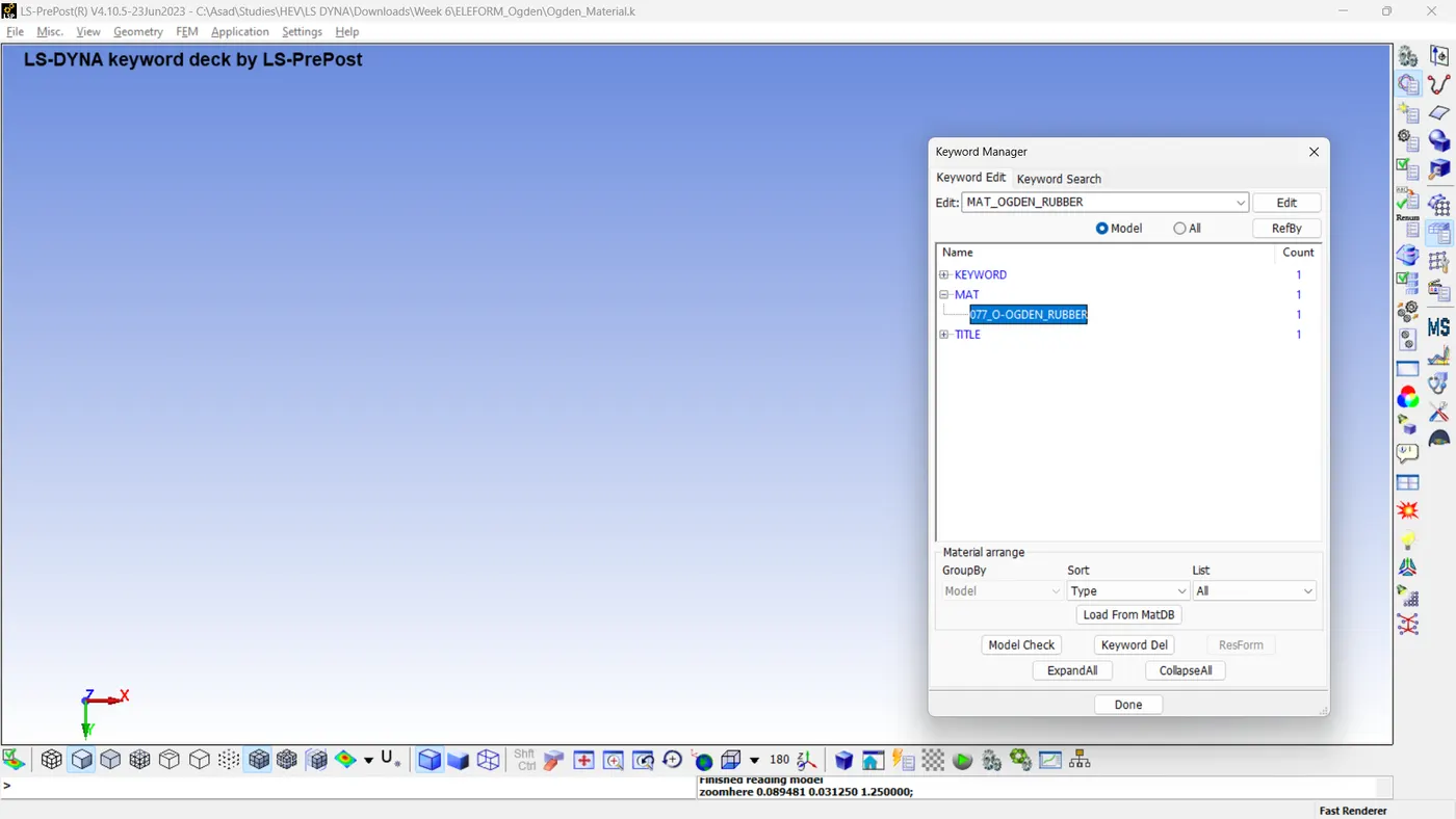
Download the keyword file and save it in a suitable location. Open LS-Prepost and load the keyword file (.K format). Open the keyword manager and understand the model with the assistance of the keyword manager.

Step 02: Creating a 10x10x10 Cube FEM Model

The model currently includes only a material card defined with Ogden material properties. According to the objective, a cube should be created using hexahedral elements, with the dimensions specified as 10x10x10 mm. The desired outcome can be realized by adhering to the following steps.

• Element and Mesh >> Shape Master >> Entity = Box Solid >> GenSelect = Region >> Define the min and max positions in X, Y and Z direction (0,0,0) and (10,10,10) >> Define the no. of elements in X, Y and Z direction (Vx, Vy and Vz) = 10, with step size =1. >> Give Target Name >> Set other options as default >> Create >> Done.

1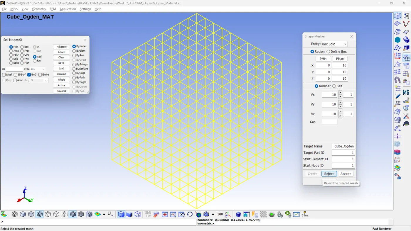

Step 03: Defining Sections

The primary goal is to compute and contrast the stretch ratio using different element formulations (-2, -1, 1 and 2). Initially, a section is defined using ELFORM=1, and the process is carried forward. Ultimately, the ELFORMs can be altered, and those models can be saved separately.

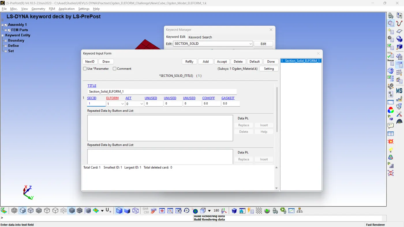
• Model A: ELFORM =1
• Model B: ELFORM =-1
• Model C: ELFORM =2
  
• Model D: ELFORM =-2
  

Step 04: Assigning Material And Section Cards To The Part

The Ogden material card has been predefined in the model with appropriate material properties. Additionally, the models utilizing ELFORM 1 and -1 require hourglass stabilization and control. Therefore, it is necessary to define an hourglass card for both models and assign it to the respective parts for Model A and Model B.

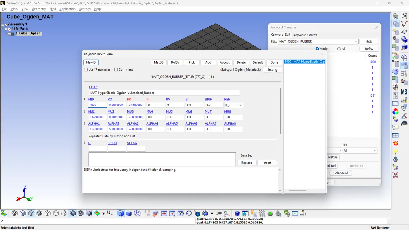
Then, assign the material and section card to the part.

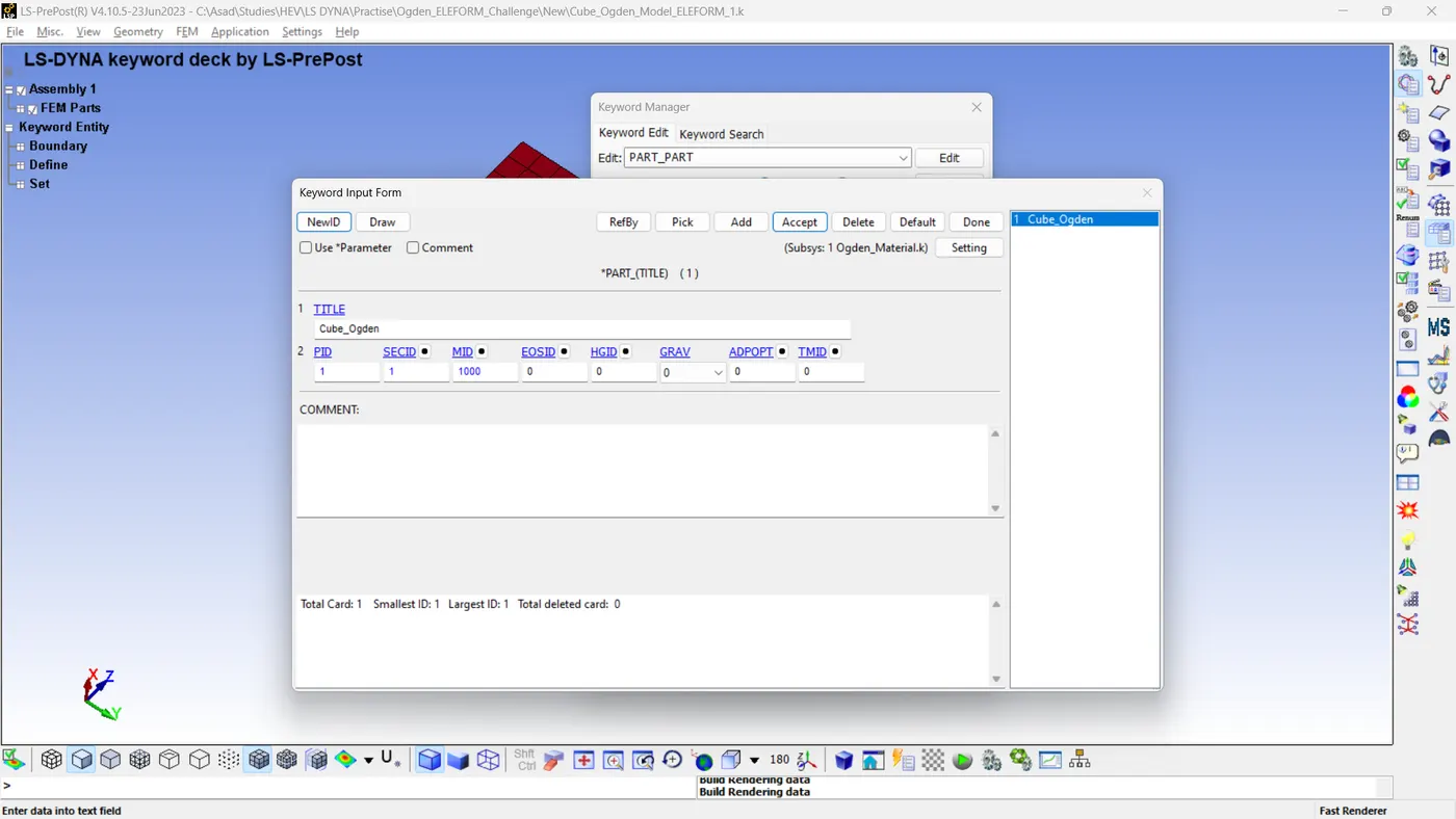
Step 05: Setting Boundary Conditions

Here, we need to simulate a tensile test in the X-direction. For that, we need to restrict the motion of nodes in the outermost part of the cube in the YZ plane. Initially, node sets must be created. The first set will include all the nodes on the bottom plane, which restrict motion in the X direction and prevent other rotations. Similarly, we need to generate two sets that include the mid-nodes in the lower and upper sections. These nodes must be positioned on the XY and XZ planes and saved separately. For the specified motion, create a node set that encompasses the nodes on the top section of the cube in the YZ plane.

1. SPC_X_Restricted
2. SPC_Y_Restricted
   
3. SPC_Z_Restricted
   
4. SPC_BPM_X

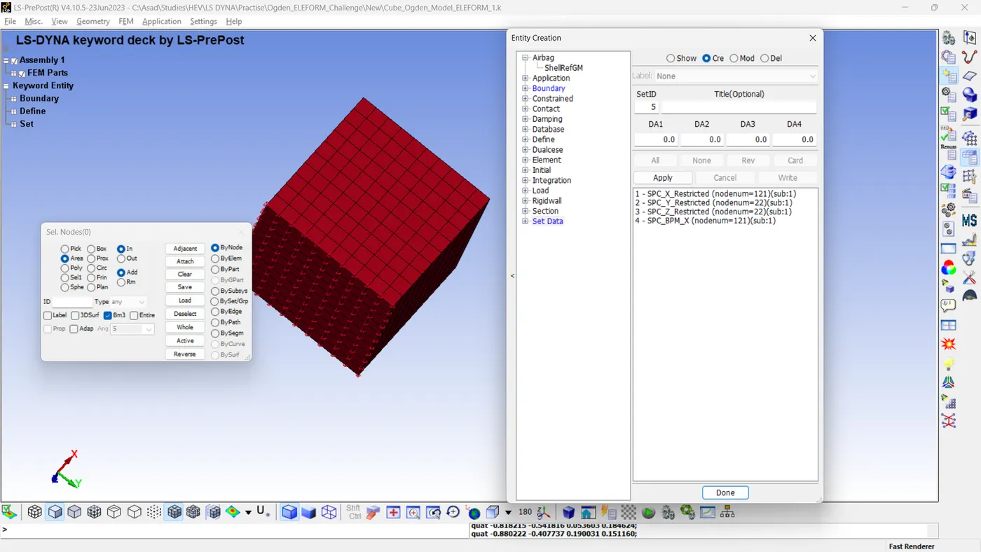
The boundary condition should be applied as mentioned below.

1. X_Constrained:- DOFX, DOFRX, DOFRY and DOFRZ are constrained.
2. Y_Constrained:- DOFY is constrained.
   
3. Z_Constrained:- DOFZ is constrained
   

• Model And Part >> Keyword Manager >> All >> Boundary >> SPC_SET >> Select suitable NSID and DOF Options >> Accept >> Done.
  

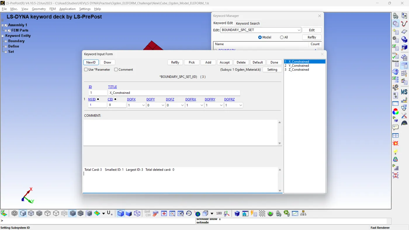
Step 06: Defining Prescribed Motion

The displacement should be assigned using the prescribed motion. For that, we need to define a curve.

We know that,

True Strain = ln (1+ Engineering Strain)

And Stretch Ratio = 1+Engineering Strain

= 1+ (dL/L)

As per the question,

Maximum stretch ratio = 5,

Initial Length, L = 10mm

So, dL = (5-1)*10

= 40mm.

The table illustrates the relationship between simulation time and the change in length. Using this data, define a curve.

A1	O1
0	0
2	40
2.5	40

• Model And Part >> Keyword Manager >> All >> Define >> Curve >> LCID=1 >> Give The Data For The Curve Definition >> Plot >> Accept >> Done.
  

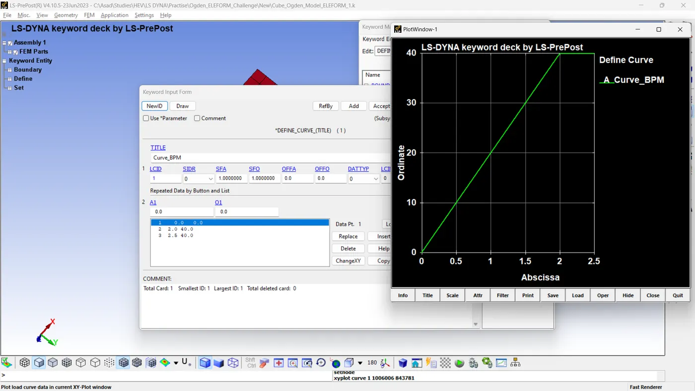
Subsequently, utilizing the curve data, we must implement a prescribed motion to the top nodes in the X direction.

• Model And Part >> Keyword Manager >> All >> Boundary >> Prescribed Motion Set >> Give ID and Title >> Select NSID (Nodes On Top Side) >> DOF = 2 (X directional DOF) >> VAD = 2 (displacement) >> LCID=1 (Select Curve ID) >> Accept >> Done.
  

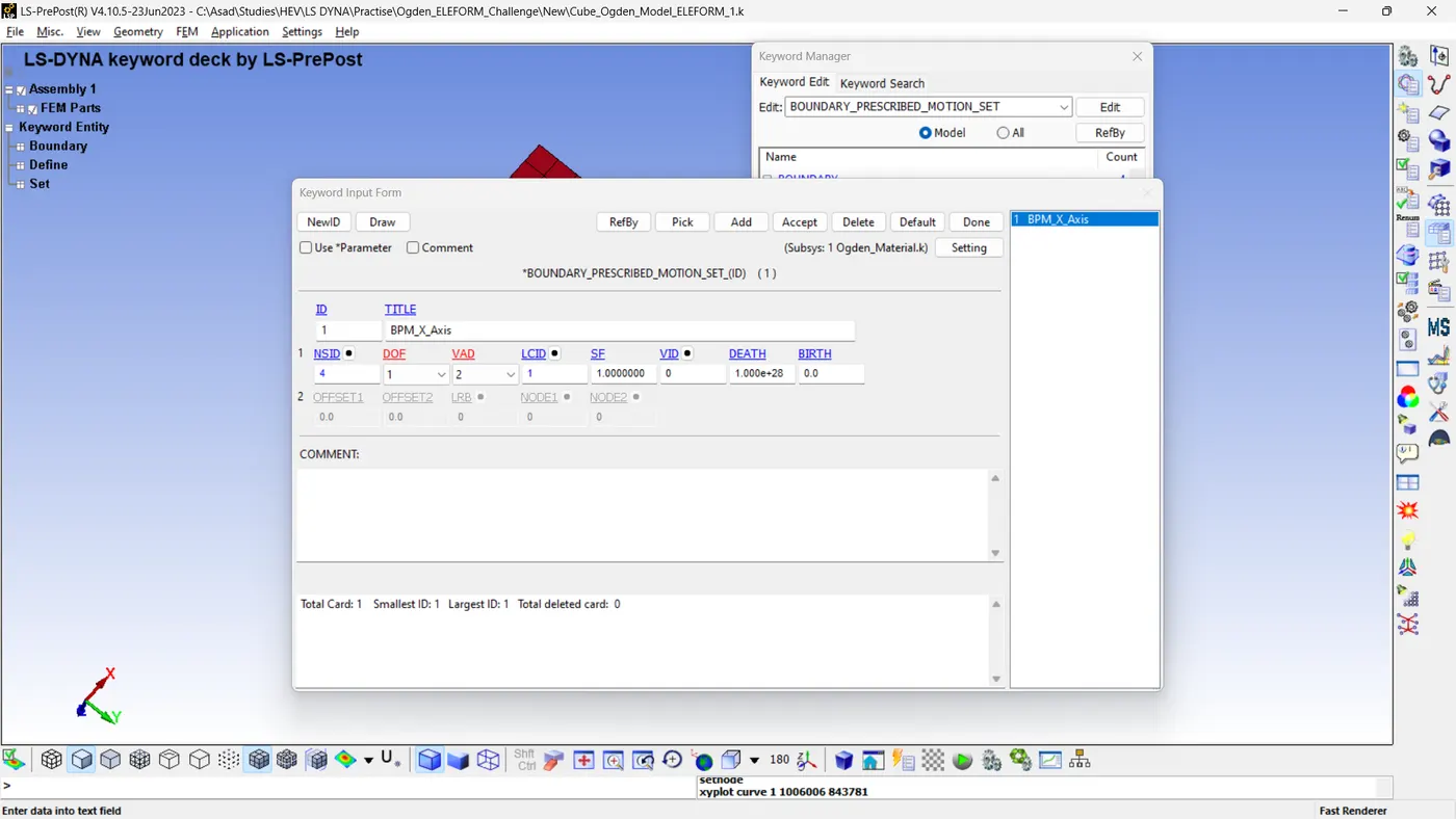
Step 07: Defining Control Cards

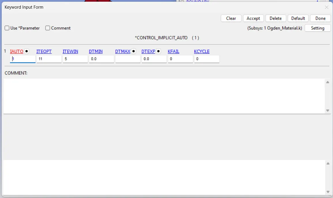
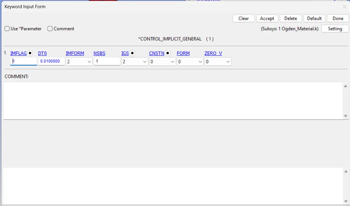
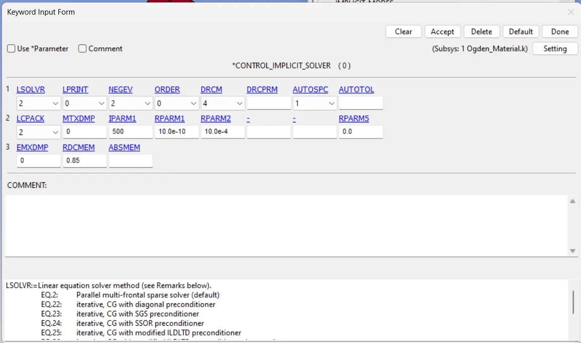
The termination card must be defined with ENDTIM=2ms. Because we conduct implicit analysis, it is necessary to define implicit control cards. The following implicit cards should be defined with appropriate values to conduct the implicit simulation

1. Control_Implicit_Auto

2. Control_Implicit_General

3. Control_Implicit_Solution

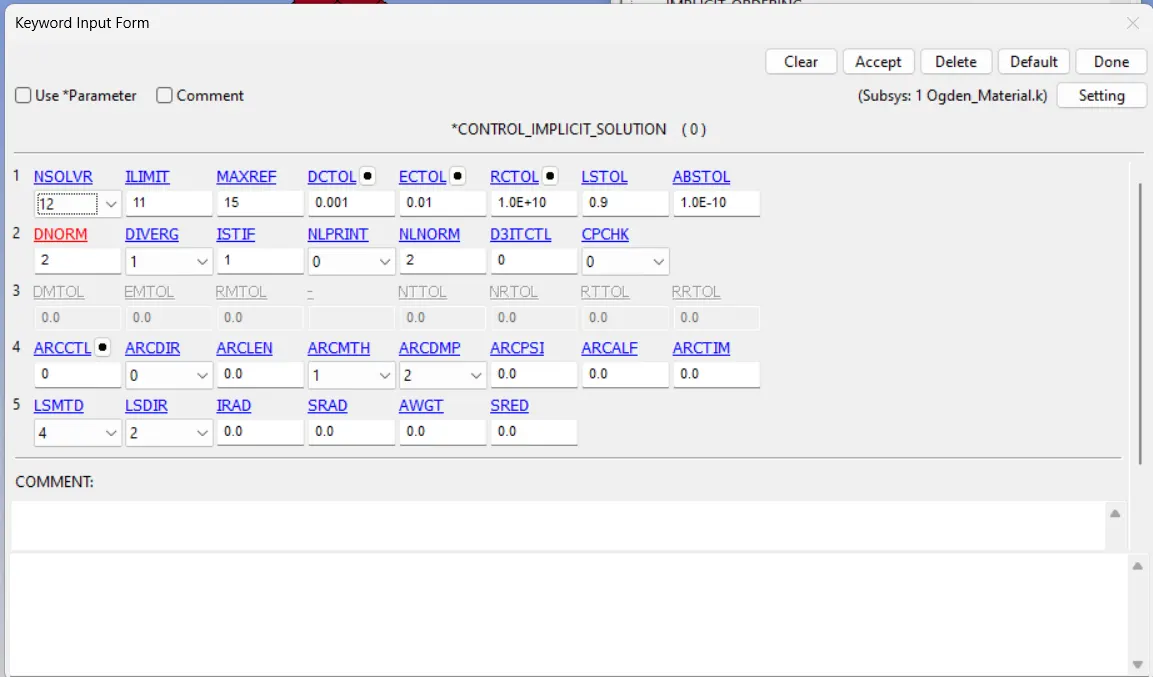
4. Control_Implicit_Solver

Step 11: Requesting Outputs

Per the objective, we need D3PLOT as a binary output with DT=0.1ms. Additionally, it is necessary to activate the EXTENT_BINARY database card to manage the content of the binary output databases d3plot, d3thdt, and d3part to a certain degree. We need to enable STRFLG =1. This setting allows the output of true strain rates to be written directly to the output databases.

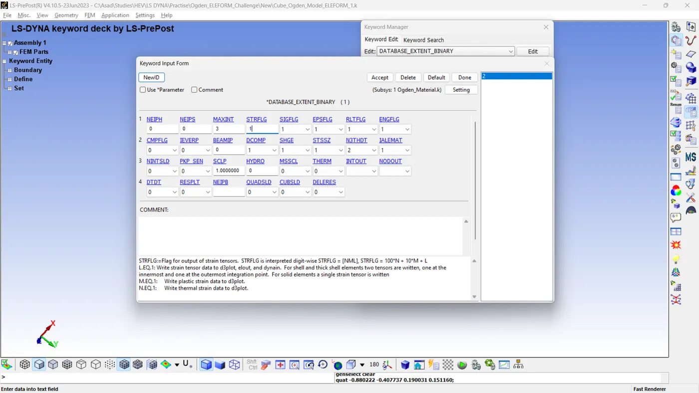
There's no need to enable major ASCII outputs or other database cards if extracting those outputs is unnecessary.

Step 12: Model Checking And Simulation For Each Case

Model checking should be finalized, and any errors identified within the model must be resolved.

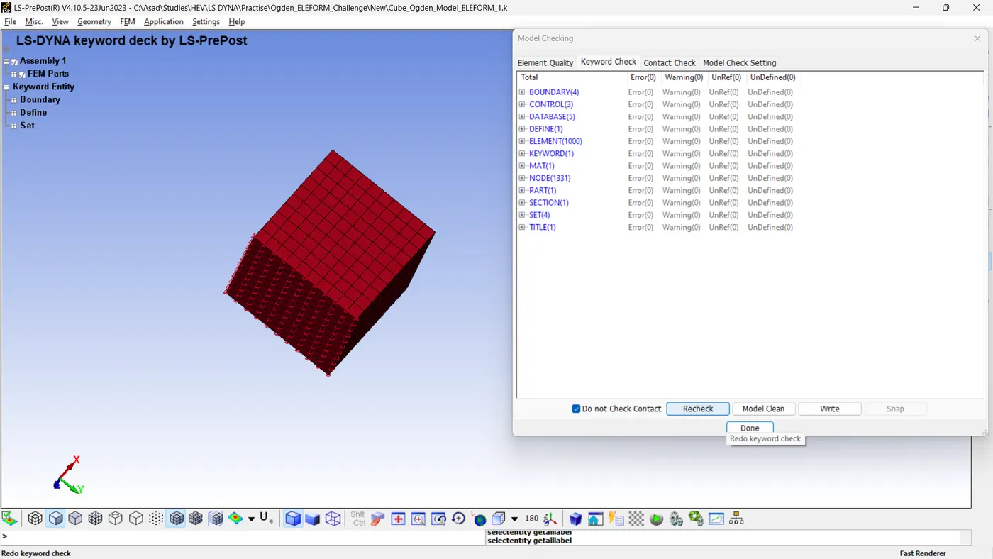
Save the file with an appropriate name and a '.K' extension. Adjust the element formulation values to 2, 1, -1, and -2, then save and execute the simulations individually.

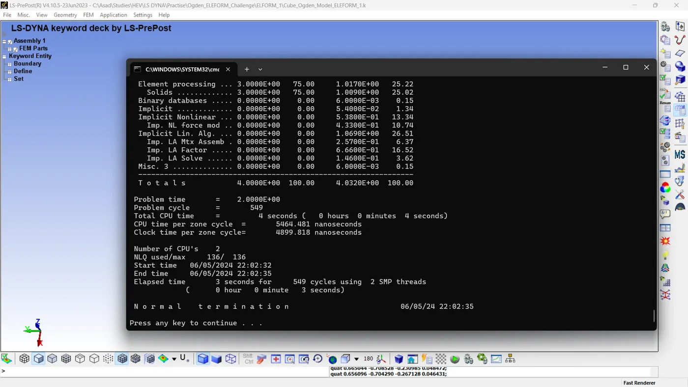
Results

According to the deliverables, we must compute the engineering stress and strain values for each time step based on the true stress and strain values provided in the output file. Subsequently, we need to determine the stretch ratio, plot the engineering stress versus stretch ratio graph, and analyze the results.

The equations utilized for the calculations are as follows.

• Engineering Strain = (exp(True Stress))-1
• Stretch Ratio = 1+Engineering Strain
• Engineering Stress = True Stress/(1+Engineering Strain)

Model A: ELFORM = 1

For ELFORM = 1, it represents a single-point integration with hourglass control. This is the default setting for solid elements in LS-DYNA. Here are some characteristics of this formulation:

• It is efficient and accurate.
• It can sustain large nonlinear deformations.
• It requires hourglass control.
• The choice of hourglass formulation and values remains an issue.

This formulation is often used for modelling solid bodies and structures without any a priori geometric simplification. It treats boundary conditions more realistically compared to shells or beams. However, it requires more effort in terms of mesh preparation, CPU time, and post-processing.

Please note that the use of ELFORM = 1 might require you to adjust the hourglass control parameters in the HOURGLASS command to prevent spurious zero-energy deformation modes.

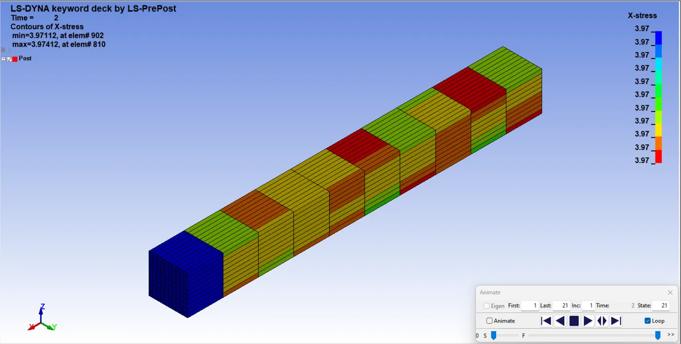
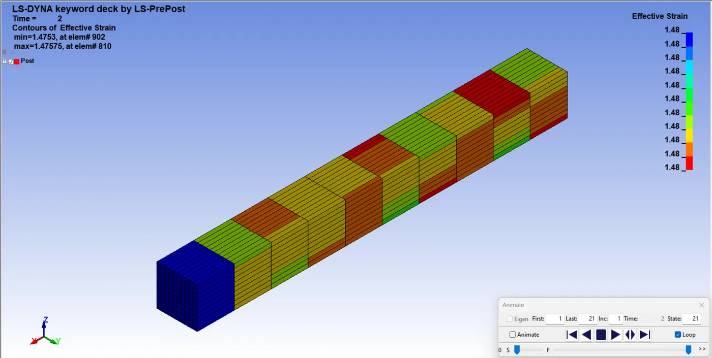
The table below displays the engineering stress, strain, and stretch ratio derived from the true stress and strain values.

Model A: ELFORM = 1
Time	True Strain	True Stress	Engineering Strain	Stretch Ratio	Engineering Stress
0	0	0	0	1	0
0.15837	0.258582	0.344209	0.295092343	1.295092343	0.265779504
0.25837	0.3949	0.548784	0.48423576	1.48423576	0.369741799
0.35837	0.513586	0.74447	0.671273649	1.671273649	0.44545069
0.45837	0.618645	0.934611	0.8564109	1.8564109	0.503450502
0.55837	0.71258	1.12077	1.039245731	2.039245731	0.549600268
0.65837	0.797693	1.30614	1.220412523	2.220412523	0.588242043
0.75837	0.874931	1.48985	1.398709777	2.398709777	0.621104735
0.85837	0.946634	1.67665	1.577020792	2.577020792	0.650615628
0.95837	1.01204	1.8634	1.751207758	2.751207758	0.677302539
1.05837	1.07139	2.04874	1.919434695	2.919434695	0.701759147
1.1539	1.12728	2.23943	2.087247756	3.087247756	0.72538072
1.2539	1.17935	2.43343	2.252259547	3.252259547	0.748227491
1.3539	1.22941	2.63796	2.419211606	3.419211606	0.771511186
1.4539	1.27318	2.83131	2.572194097	3.572194097	0.792596909
1.5539	1.31564	3.03517	2.727135589	3.727135589	0.814343865
1.6539	1.35554	3.24229	2.878854973	3.878854973	0.835888432
1.7539	1.39274	3.45088	3.025865827	4.025865827	0.857177101
1.8539	1.42787	3.6621	3.169808035	4.169808035	0.878241868
1.9539	1.46156	3.881	3.312682067	4.312682067	0.899904036
2	1.47575	3.97447	3.374315279	4.374315279	0.908592487

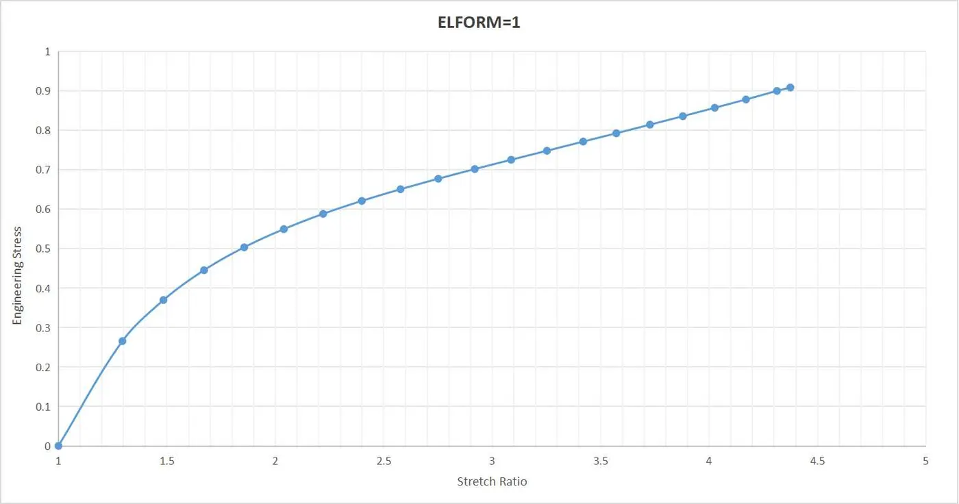
Displayed below is the plot of engineering stress versus stretch ratio.

Model B: ELFORM = -1

In LS-DYNA, the element formulation -1 for SECTION_SOLID is a fully integrated S/R solid intended for elements with poor aspect ratio. This formulation is efficient. Solid elements in LS-DYNA are three-dimensional finite elements that can model solid bodies and structures without any a priori geometric simplification. They treat boundary conditions more realistically compared to shells or beams.

However, it’s important to note that while this formulation is efficient, it may require a higher effort in terms of mesh preparation, CPU time, and post-processing. It might also perform poorly for thin-walled structures due to locking problems.

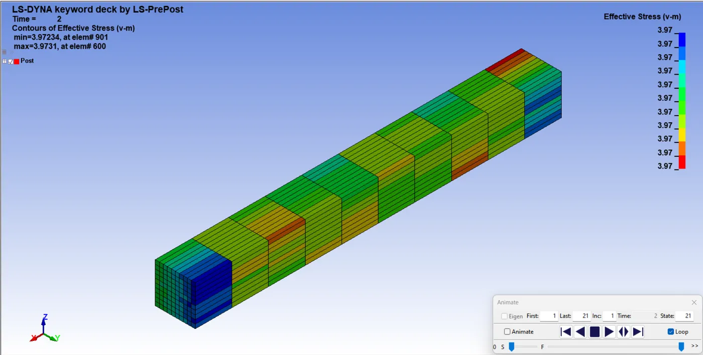
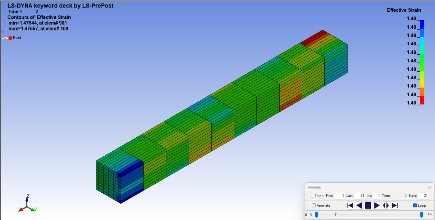
The table below displays the engineering stress, strain, and stretch ratio derived from the true stress and strain values.

Model B: ELFORM = -1
Time	True Strain	True Stress	Engineering Strain	Stretch Ratio	Engineering Stress
0	0	0	0	1	0
0.15837	0.258581	0.344207	0.295091048	1.295091048	0.265778225
0.25837	0.394897	0.54878	0.484231307	1.484231307	0.369740213
0.35837	0.513584	0.744468	0.671270307	1.671270307	0.445450384
0.45837	0.618622	0.934565	0.856368203	1.856368203	0.503437302
0.55837	0.71275	1.12153	1.039592433	2.039592433	0.549879467
0.65837	0.79789	1.3063	1.220849988	2.220849988	0.588198216
0.75837	0.87589	1.49343	1.401011243	2.401011243	0.622000419
0.85837	0.946236	1.67595	1.575995342	2.575995342	0.650602885
0.95837	1.01226	1.86391	1.75181309	2.75181309	0.677338881
1.05837	1.0714	2.04873	1.91946389	2.91946389	0.701748704
1.1539	1.12853	2.24342	2.091109228	3.091109228	0.725765359
1.2539	1.17972	2.43474	2.253463106	3.253463106	0.748353346
1.3539	1.2278	2.63037	2.413711105	3.413711105	0.770530932
1.4539	1.27317	2.83099	2.572158375	3.572158375	0.792515253
1.5539	1.31572	3.03561	2.727433772	3.727433772	0.814396764
1.6539	1.35538	3.24158	2.878234406	3.878234406	0.835839112
1.7539	1.39275	3.45101	3.025906086	4.025906086	0.857200821
1.8539	1.42803	3.66319	3.170475258	4.170475258	0.878362722
1.9539	1.46095	3.87435	3.310052134	4.310052134	0.898910241
2	1.47557	3.9731	3.373527974	4.373527974	0.9084428

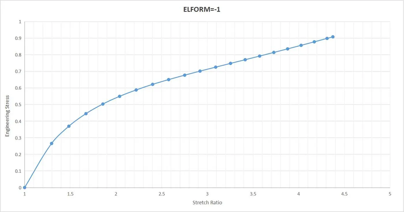
Displayed below is the plot of engineering stress versus stretch ratio.

Model C: ELFORM = 2

In LS-DYNA, the element formulation ELFORM=2 refers to a fully integrated selective reduced integrated brick element. Here are some key characteristics of this formulation:

• It alleviates volumetric locking.
• No hourglass stabilization is needed.
• It is slower than ELFORM=1.
• It can be too stiff in many situations, especially for poor aspect ratios (shear locking).
• It can be more unstable in large deformation applications.

Solid elements in LS-DYNA are three-dimensional finite elements that can model solid bodies and structures without any a priori geometric simplification. They treat boundary conditions more realistically compared to shells or beams. However, the ELFORM=2 formulation can be more challenging to use due to its potential stiffness and instability in certain situations.

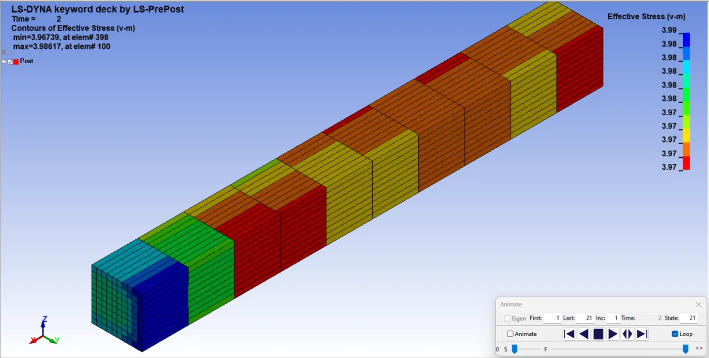
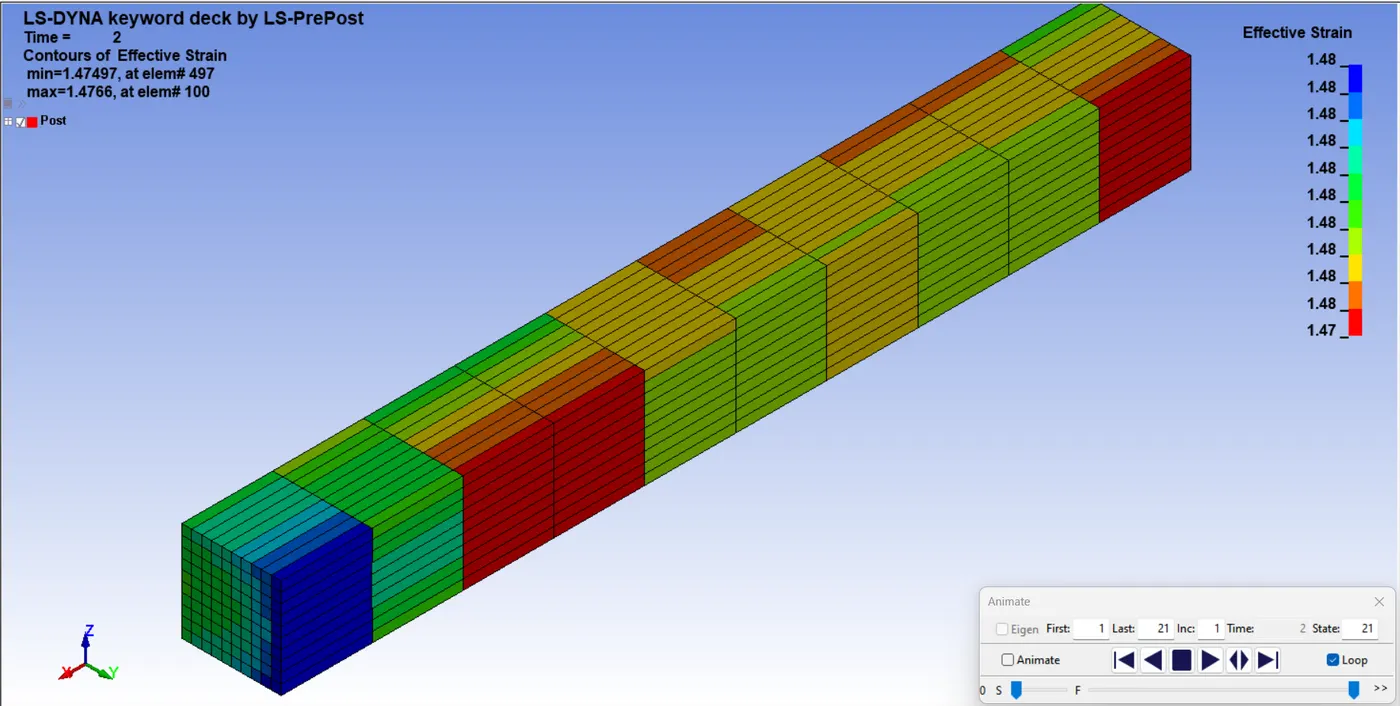
The table below displays the engineering stress, strain, and stretch ratio derived from the true stress and strain values.

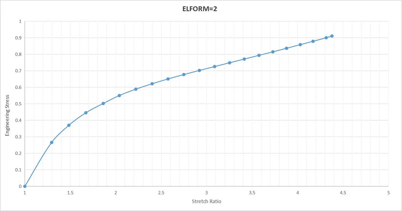
Model C: ELFORM = 2
Time	True Strain	True Stress	Engineering Strain	Stretch Ratio	Engineering Stress
0	0	0	0	1	0
0.15837	0.258581	0.344207	0.295091048	1.295091048	0.265778225
0.25837	0.394897	0.54878	0.484231307	1.484231307	0.369740213
0.35837	0.513584	0.744468	0.671270307	1.671270307	0.445450384
0.45837	0.621862	0.93456	0.86239259	1.86239259	0.50180612
0.55837	0.712736	1.1216	1.039563879	2.039563879	0.549921487
0.65837	0.797724	1.30634	1.220481357	2.220481357	0.588313879
0.75837	0.875574	1.49097	1.400252644	2.400252644	0.62117211
0.85837	0.945797	1.67433	1.574864728	2.574864728	0.650259403
0.95837	1.01104	1.8604	1.748457925	2.748457925	0.676888659
1.05837	1.0713	2.04841	1.919171958	2.919171958	0.701709262
1.1539	1.12728	2.23944	2.087247756	3.087247756	0.725383959
1.2539	1.17927	2.43319	2.251999377	3.251999377	0.748213551
1.3539	1.22771	2.63031	2.413403884	3.413403884	0.770582705
1.4539	1.27405	2.83632	2.575303258	3.575303258	0.793308929
1.5539	1.31583	3.0362	2.727843812	3.727843812	0.814465453
1.6539	1.35537	3.24181	2.878195624	3.878195624	0.835906776
1.7539	1.39372	3.45775	3.029813109	4.029813109	0.858042273
1.8539	1.42787	3.66235	3.169808035	4.169808035	0.878301823
1.9539	1.46194	3.88197	3.314321198	4.314321198	0.89978697
2	1.4766	3.98617	3.378035028	4.378035028	0.910492944

Displayed below is the plot of engineering stress versus stretch ratio.

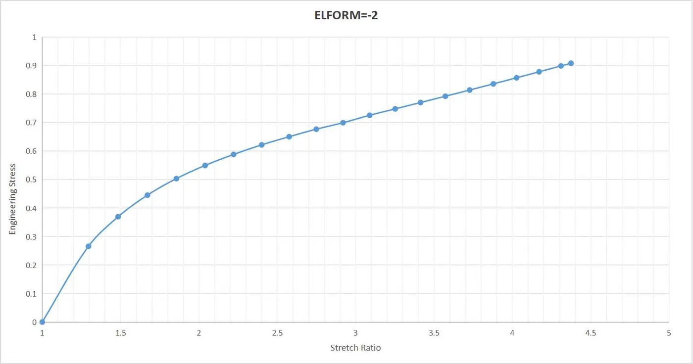
Model D: ELFORM = -2

In LS-DYNA, the element formulation ELFORM=-2 refers to a fully integrated selective reduced integrated solid intended for elements with poor aspect ratio. This formulation is identical to ELFORM=2, but it is specifically designed to account for poor aspect ratios to reduce shear locking. Here are some key characteristics of this formulation

• It is intended for elements with poor aspect ratios.
• It is an accurate formulation.
• It is fully integrated.
• It is selectively reduced and integrated.

Solid elements in LS-DYNA are three-dimensional finite elements that can model solid bodies and structures without any a priori geometric simplification. They treat boundary conditions more realistically compared to shells or beams. However, the ELFORM=-2 formulation can be more challenging to use due to its potential stiffness and instability in certain situations.

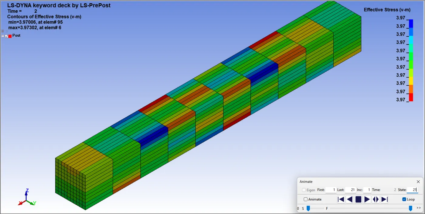
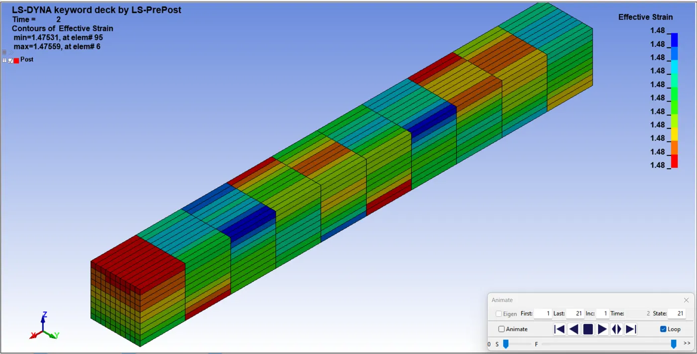
The table below displays the engineering stress, strain, and stretch ratio derived from the true stress and strain values.

Model D: ELFORM = -2
Time	True Strain	True Stress	Engineering Strain	Stretch Ratio	Engineering Stress
0	0	0	0	1	0
0.15837	0.258581	0.344207	0.295091048	1.295091048	0.265778225
0.25837	0.394897	0.54878	0.484231307	1.484231307	0.369740213
0.35837	0.513584	0.744468	0.671270307	1.671270307	0.445450384
0.45837	0.618589	0.93456	0.856306944	1.856306944	0.503451222
0.55837	0.712614	1.12109	1.039315067	2.039315067	0.549738497
0.65837	0.797897	1.30648	1.220865534	2.220865534	0.588275148
0.75837	0.875533	1.49275	1.400154235	2.400154235	0.621939198
0.85837	0.946035	1.67542	1.575477619	2.575477619	0.650527882
0.95837	1.01105	1.8606	1.74848541	2.74848541	0.676954658
1.05837	1.07121	2.04197	1.918909244	2.918909244	0.699566115
1.1539	1.12788	2.24197	2.08910066	3.08910066	0.725767868
1.2539	1.17923	2.43301	2.251869299	3.251869299	0.748188127
1.3539	1.22783	2.63079	2.413813517	3.413813517	0.770630846
1.4539	1.27317	2.83142	2.572158375	3.572158375	0.792635629
1.5539	1.31557	3.03507	2.726874699	3.726874699	0.814374039
1.6539	1.35538	3.24188	2.878234406	3.878234406	0.835916466
1.7539	1.39279	3.45158	3.026067125	4.026067125	0.857308111
1.8539	1.42792	3.66266	3.170016531	4.170016531	0.87833225
1.9539	1.46094	3.87487	3.310009033	4.310009033	0.899039879
2	1.47559	3.97302	3.373615445	4.373615445	0.90840634

Displayed below is the plot of engineering stress versus stretch ratio.

Conclusion

The tensile test was performed on a newly created 10x10x10 solid block, with each element formulation tested separately to record the true stress and strain values. These values were then used to calculate the engineering stress, strain, and stretch ratio. A graph was plotted to illustrate the relationship between the stretch ratio and engineering stress, which was then compared to the reference provided in the question to highlight the following points.

• In each instance, the plot generated was identical to the reference provided in the question. However, altering the element formulation had a negligible impact on the outcomes of strain, stress, and stretch ratios.
• In this case, the deformation is relatively minor, and the significant differences between the element formulations are not apparent.

Reference

• Ogden hyperelastic model - Wikipedia

Drive Link: https://drive.google.com/file/d/1VZyejF-Nsic_KAgPPB3Aj58pidD7JxB5/view?usp=sharing