Week-6 Calculate the Stretch Ratio by comparing the ELFORM (-2,-1,1,2) with Ogden_Material Model.

Aim : Calculate the Stretch Ratio by comparing the ELFORM (-2,-1,1,2) with Ogden_Material Model.

Procedure :

Case 1 : ELFORM 2

Open the given .k file in LS Prepost

File >> Open >> LS Dyna Keyword File

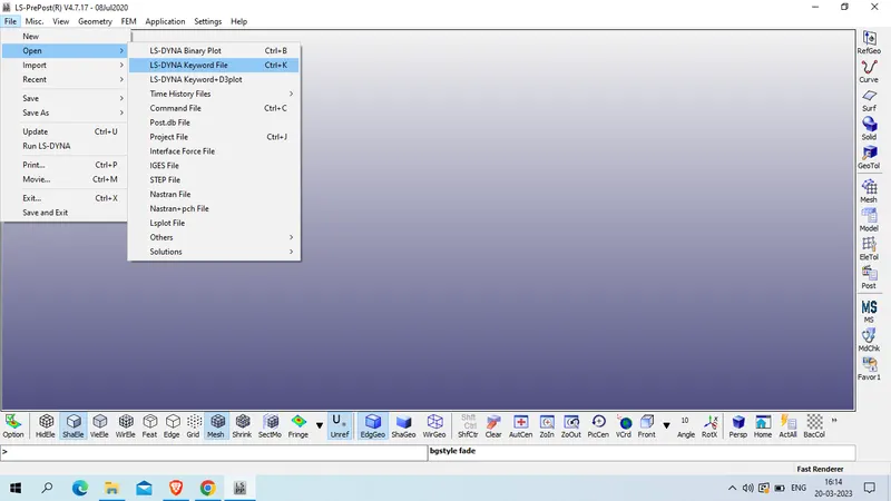
select file >> open

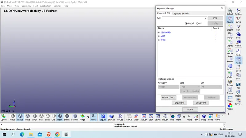
as we have data for ogden material with below data

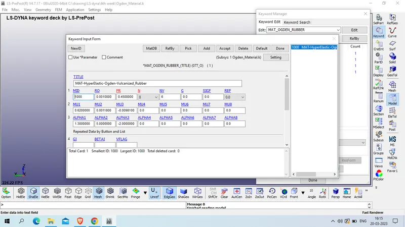
Title : MAT-HyperElastic-Ogden-Vulcanized_Rubber

MID : 1000

Density : 0.001 Kg /mm^3

Poission Ratio : 0.45

NV: 6 Default

first shear modulus. : 0.62

second shear modulus.: 0.00118

third shear modulus.: -0.00981

first exponent.: (ALPHA1) : 1.3

second exponent. : (ALPHA2) : 5.0

third exponent.: (ALPHA3) ; -2.0

now we will create 10X10X10 mm cube with 10 element on each side

go to mesh >> solid mesher

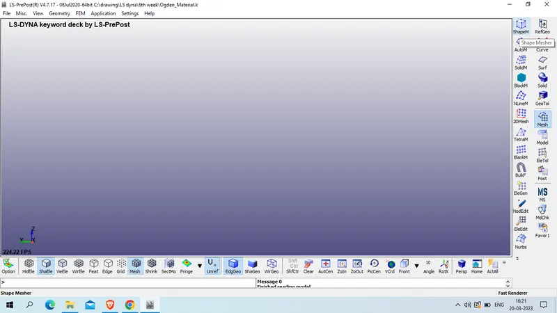
Entity : box solid

Pmax X:Y:Z :: 10

select number

Vx: 10

Vy:10

Vz: 10

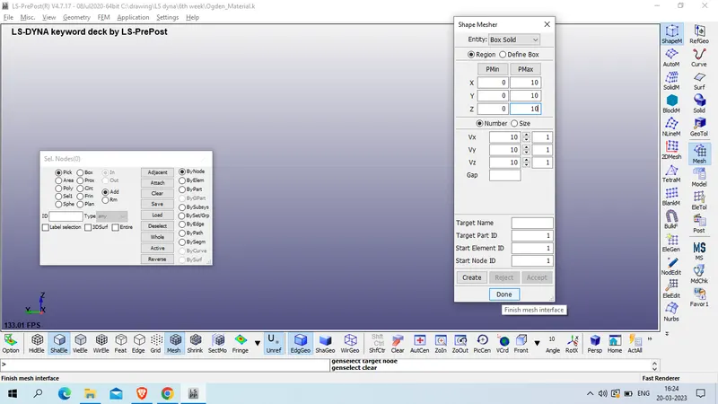
Create >> accept >> done

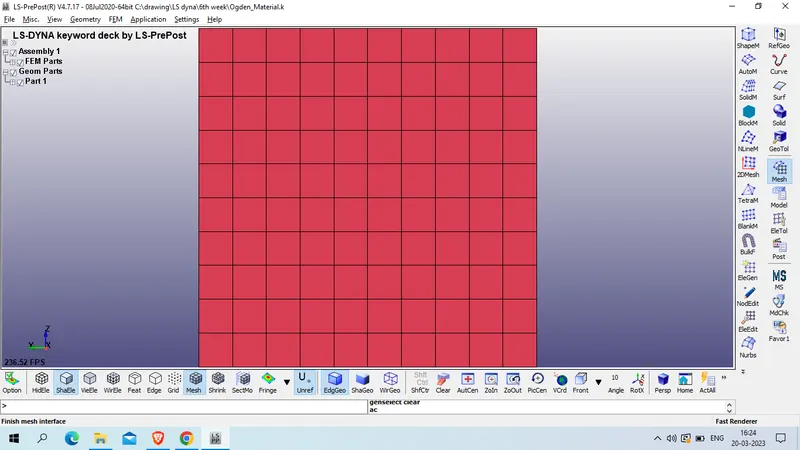
now we had successfuly created solid element , now we will create section for solid element

Model and part >> keyword manager >> all >> section >> solid

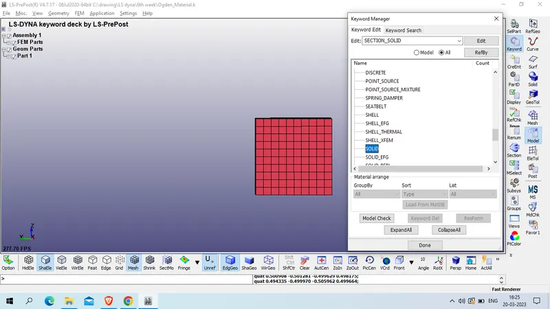
Title : Section_solid

SID : 1

ELFORM : 2 fully integrated S/R solid,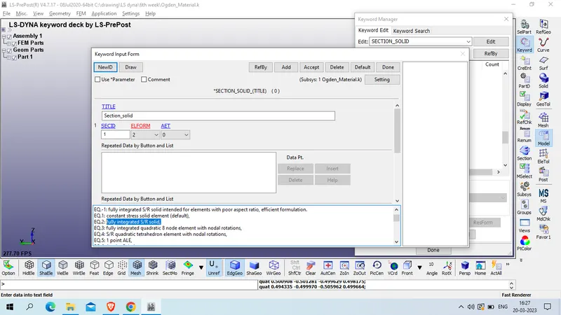

Accept >> done

Now assign section and material cart to part

Model and part >> keyword manager >> model >> part

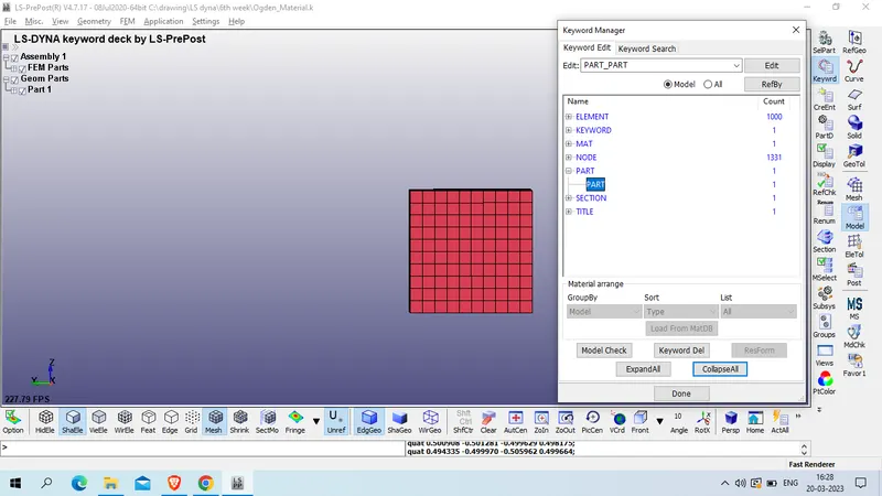
Title : CUBE_PART

PID: 1

SECID : 1 ( assign SECTION card)

MID : 1000 ( assign material card)

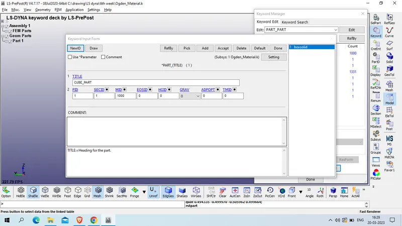
Accepty >> done

now create Boundary condition ( SPC) to fix the node

1st we will craete node set

model and part >> Create ENtity >> Set data >> Set_node

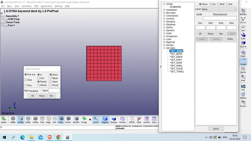
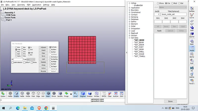
Click on create >> select node by area

Title : lower node set

select lower node set as shown below

select upper node set

title : upper_node_set

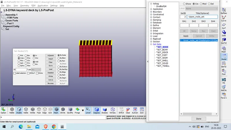
NOw select node as shown below

title : Y_ contrain

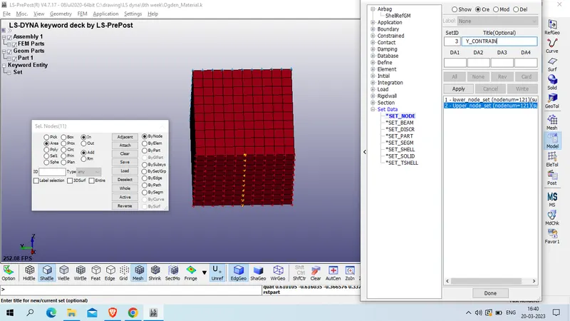
select horizontal curve as shown below

title : X_CONTRAIN

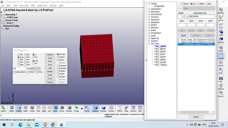
now create SPC

model and part >> create entity >> boundary condition >> SPC

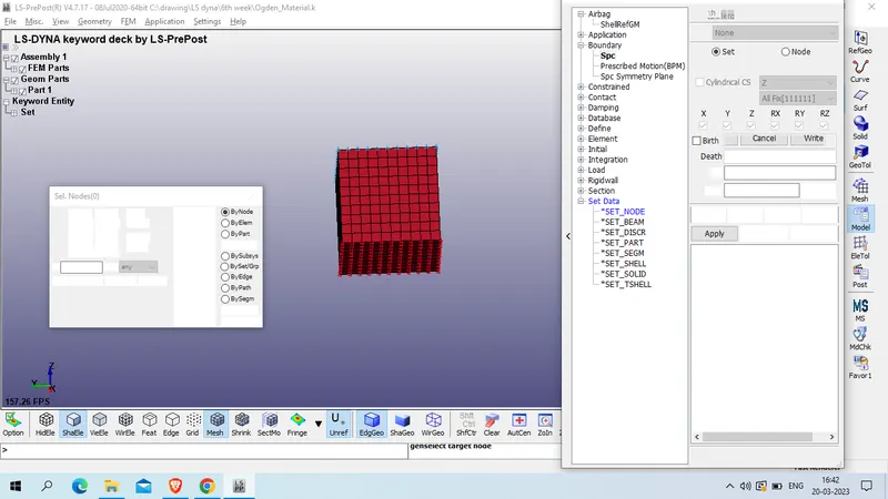
Click on create >> Set>> in NSID >>select LOWER NODE SET

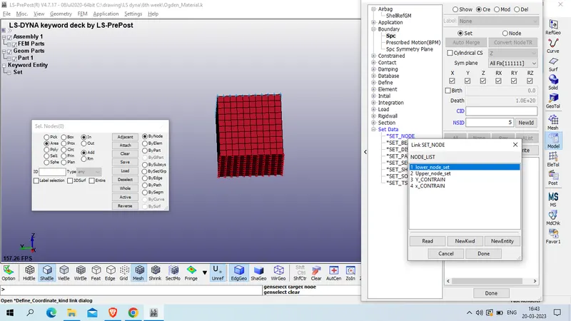
check z so that all lower node will contrained in z axis

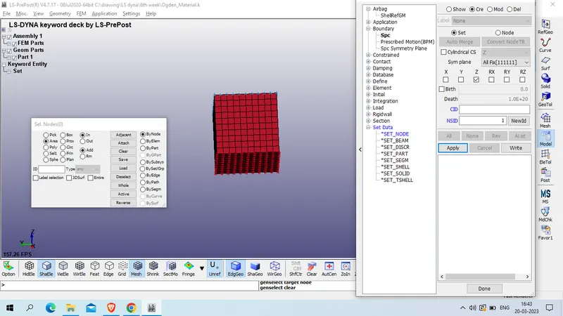
now select Y constrain node set

Check on Y to fix the node in Y movement

And after that select NSID : X CONSTRAIN

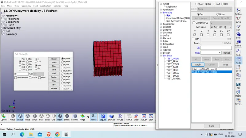
and check x box so that lower node it will not move in x axis also so that our cube wil be fix at center.

now create prescribe motion set to the upper node .

as we have to create stretch ratio 5

and we know that stretch ration = 1 + engg. strain

5 = 1 + Change in length ( L0) / Original length (10)

4= L0/10

L0 = 40

now we will create load curve for displacement upto 40 mm

model and part >> keyword manager >> all >> define >> curve

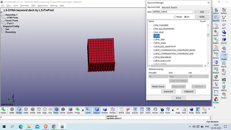
Title : DISC_CURVE

LCID : 1

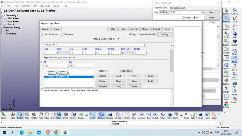
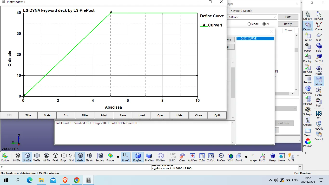
NOw Accept curve >> done

now define prescribe_Motion_set

model and part >> create entity >> boundary >> Priscribe Motion

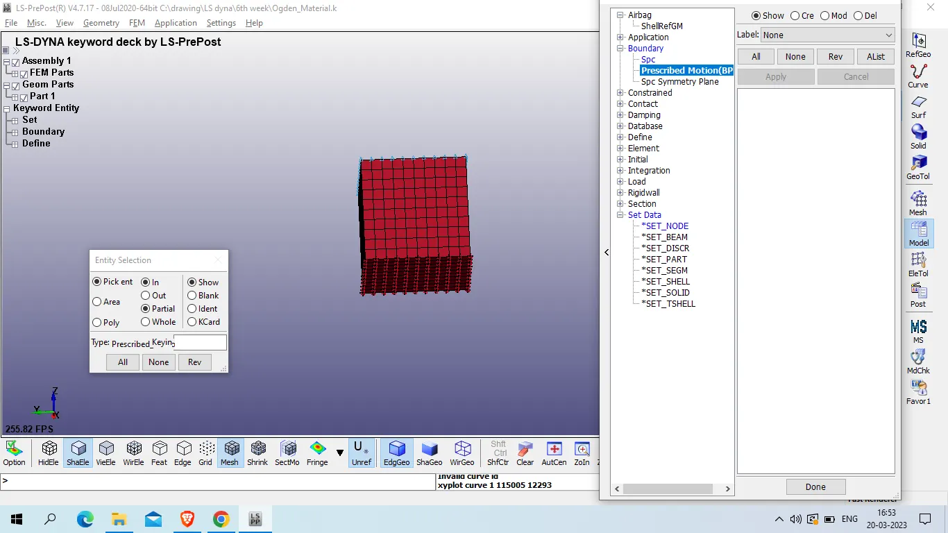
Click on create >> TYpe : set >>In NSID select upper node set

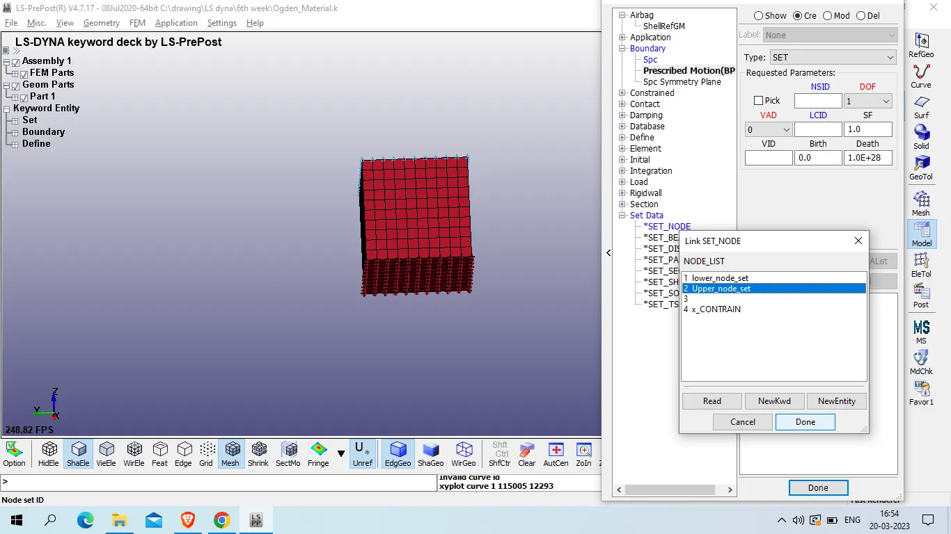
DOF : 3

VAD : 2 ( displacement )

LCID : 1 ( curve)

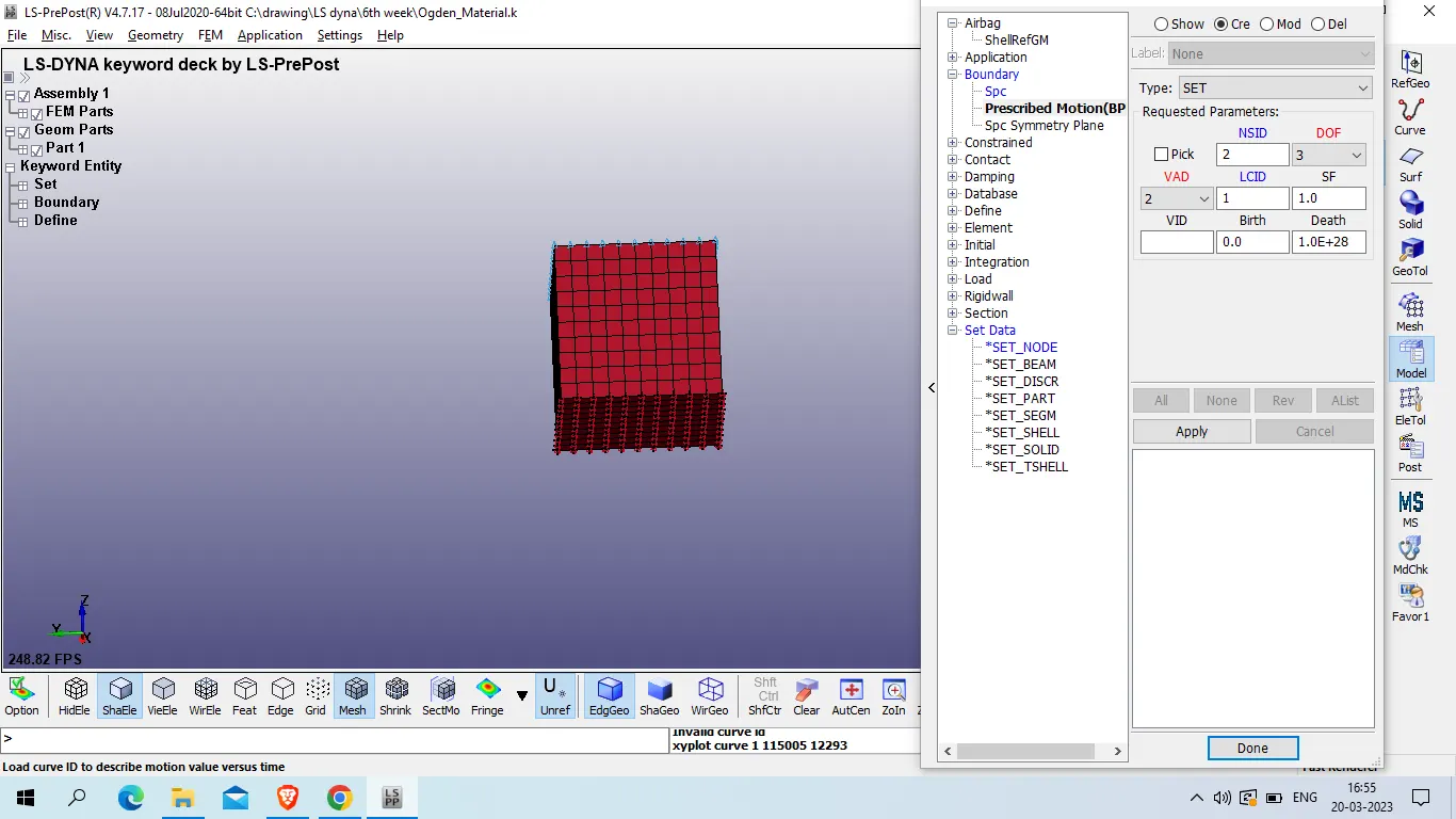
apply >> done

as we had defined boundary comtion now we will define control card , here we will use implicit analysis as we know the time is 10 ms

Since this simulation is happening at a really slow pace (quasi static) the inertial effects can be neglected we can consider implicit for the analysis.

Define Implicit cards.

1. Implicit auto

Model and part >> keyword manager >> all >> control >> implicit_auto

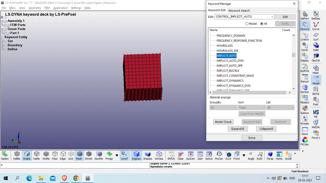
Automatic time step control flag : IAUTO : 1

ITEOPT: 100

ITEWIN: 5 (default

DTMIN: 0.001

DTMAX: 0.1

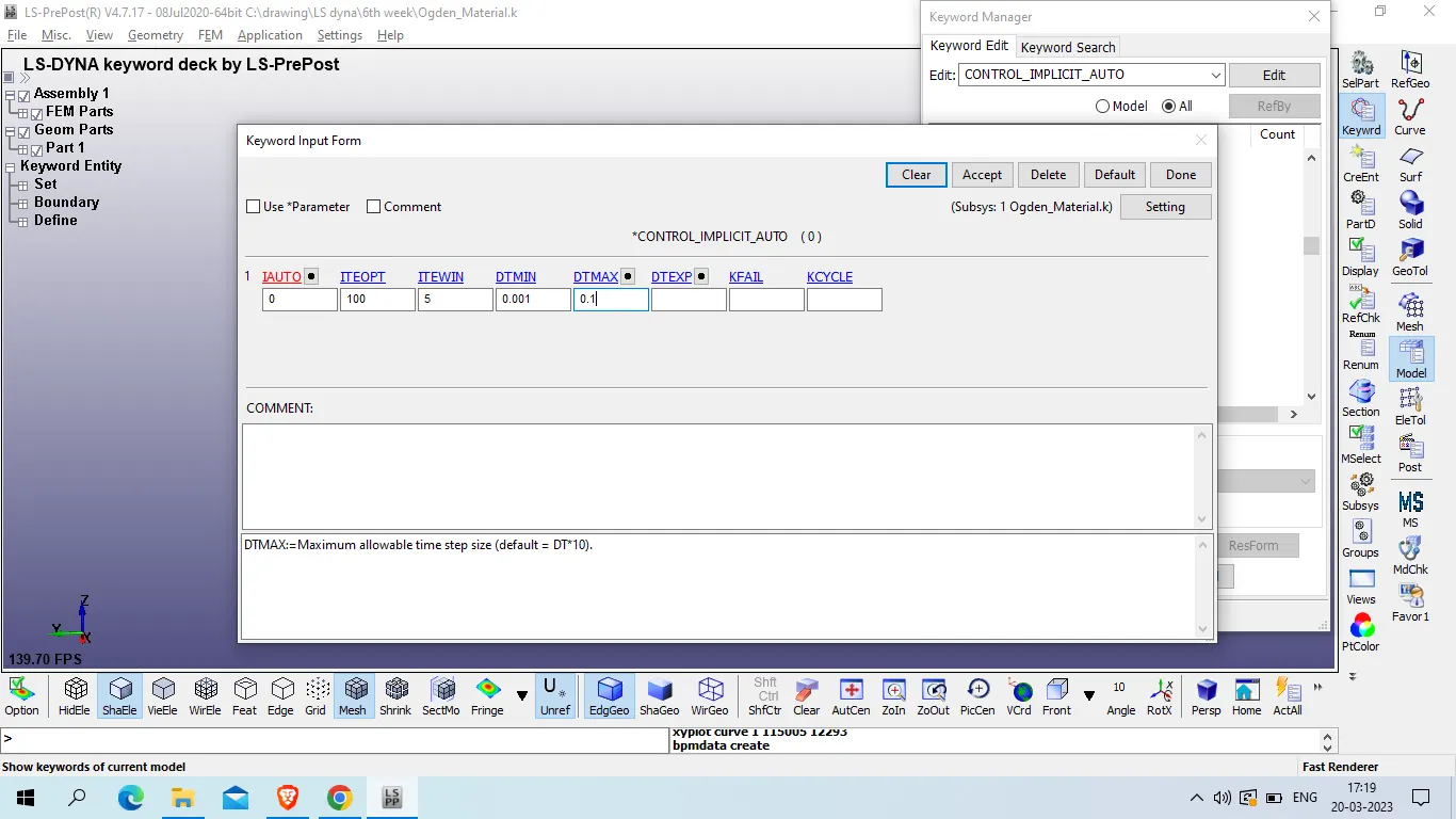
accept >> done

Now define IMplicit General card

model and part >> keyr=word manager >> all >> control >> implicit_general

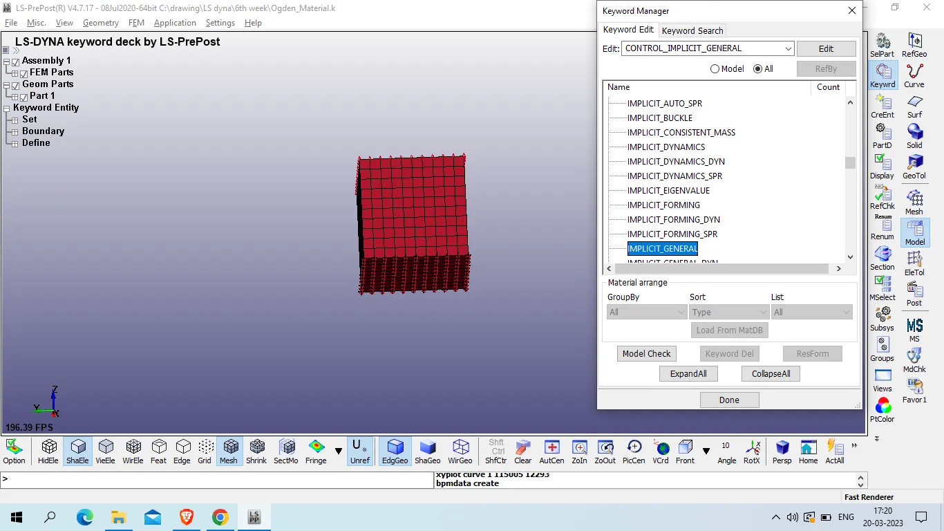
IMFLAG : 1

DT : 0.01

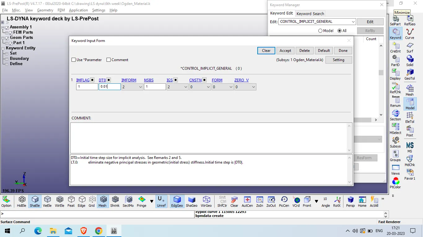
Accept >>done

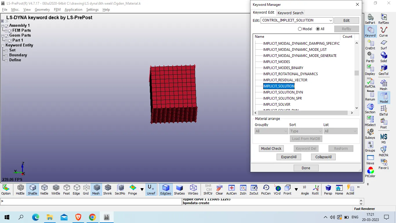
Now implicit solution

Model and part >> keyword manager >> all >> control >> Implicit_solution

NSOLVER : 12 ( Nonlinear with BFGS updates + optional arclength)

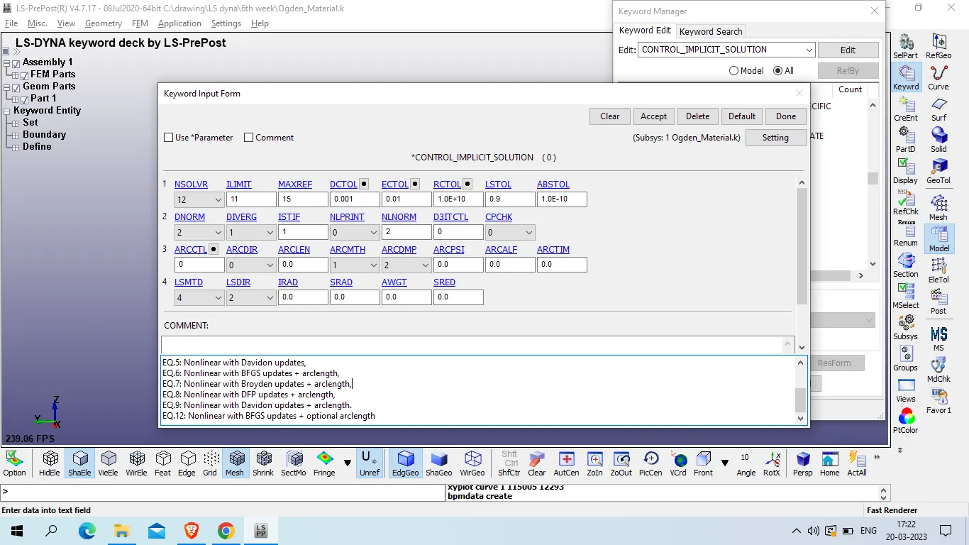
Accept >> done

Now define termination card

Model and part >> keyword manager >> all >> control >> termination

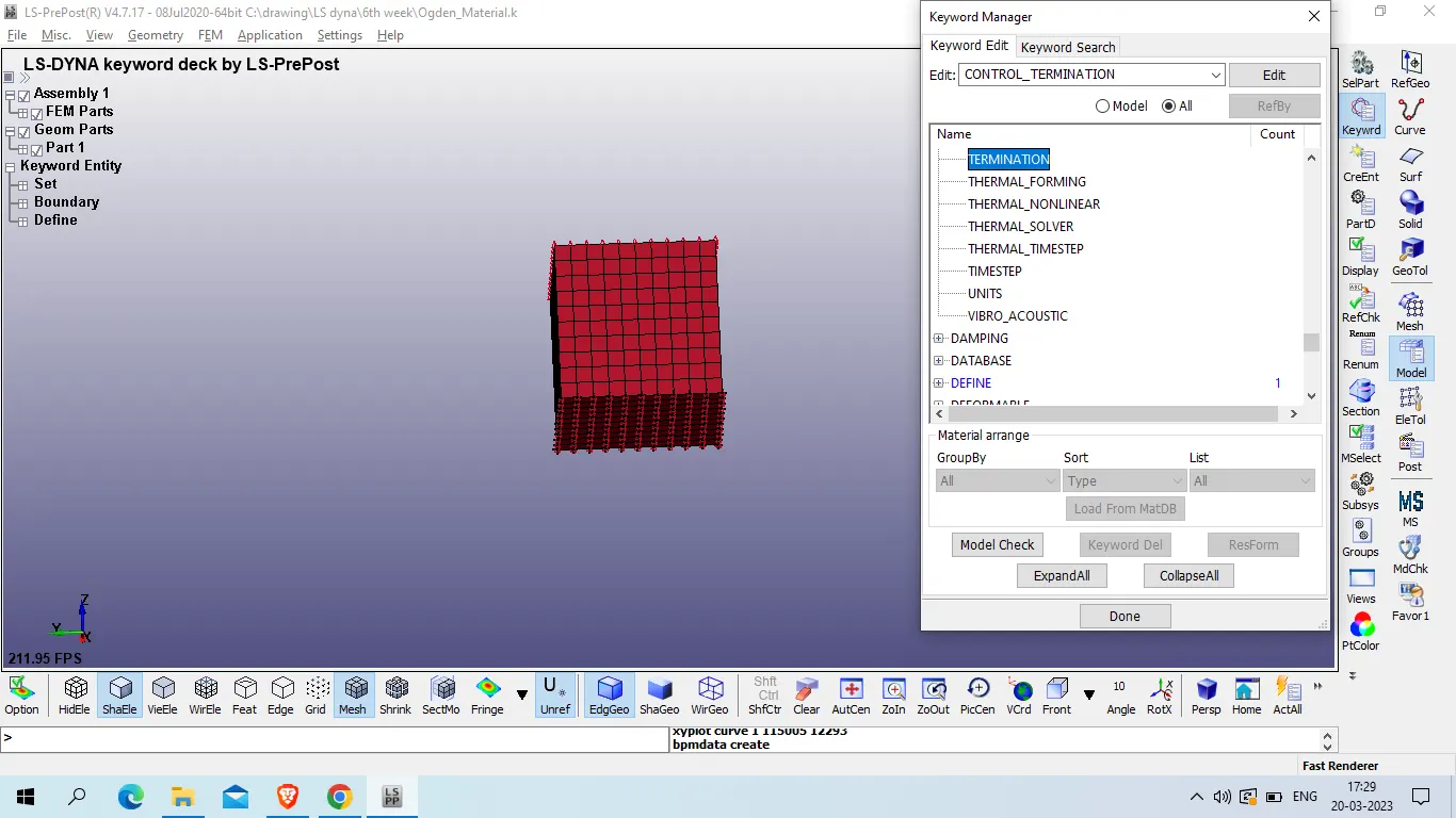
ENDTIM : 10

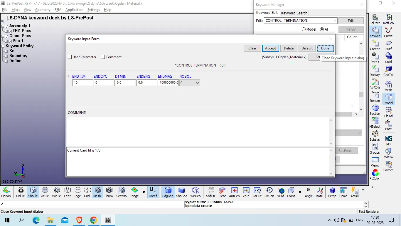
accept >> done

Model and part >> keyword manager >> all >> database >> extend_binary

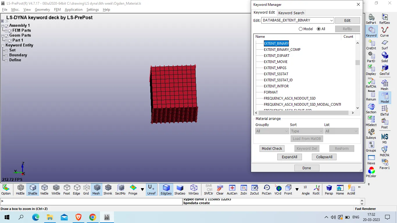
STRFLG: 1

rest are default

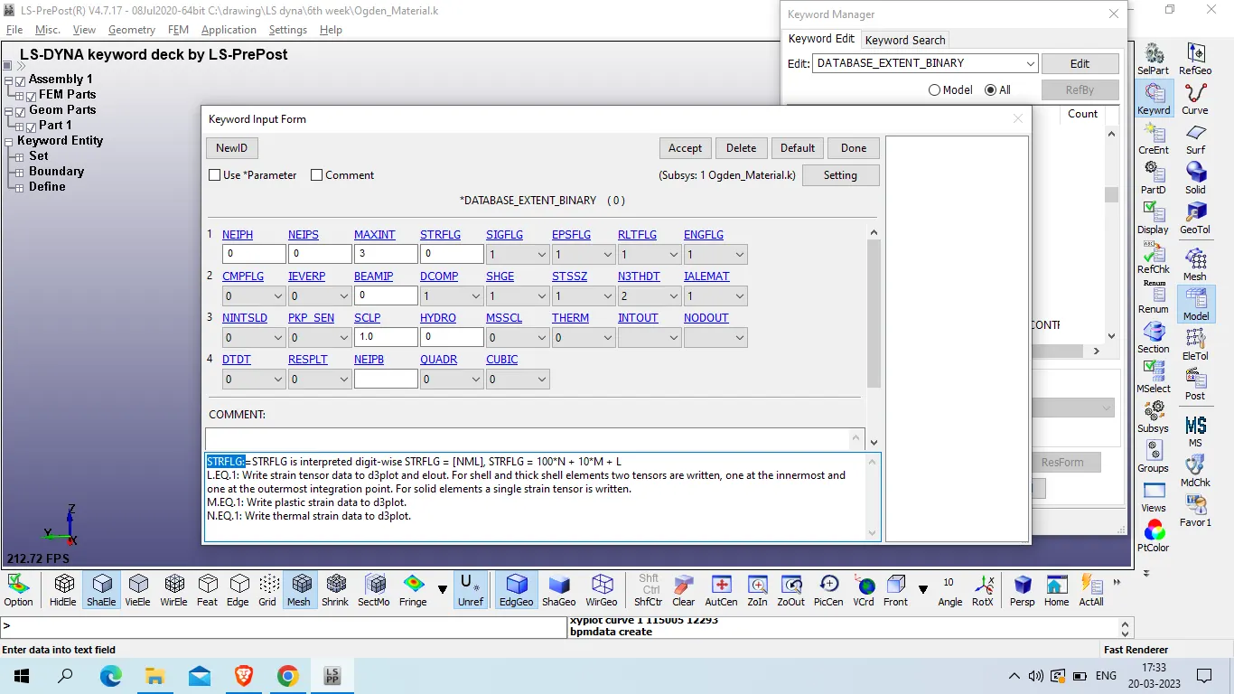
accept >> done

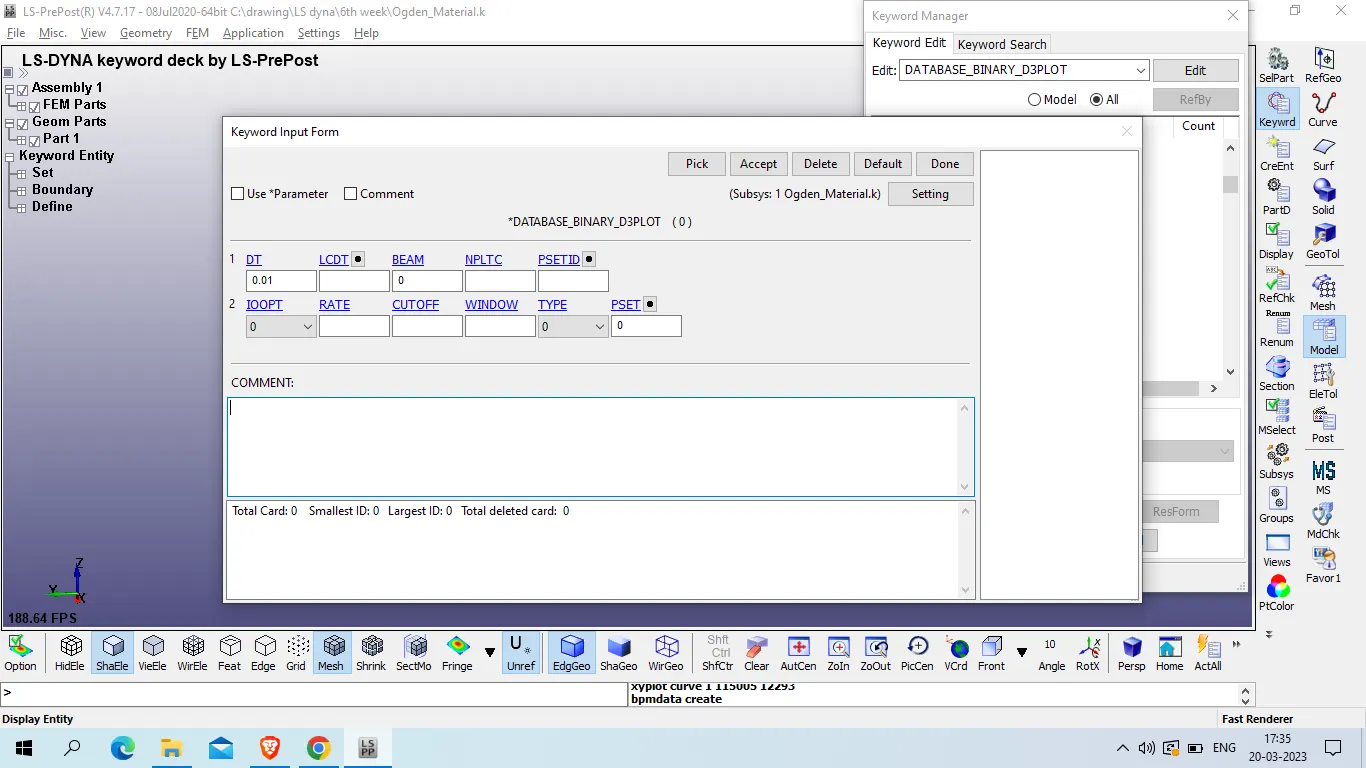
now define output in database card , Binary_d3plot card

Model and part >> keyword manager >> all >> database >> binary_d3Plot

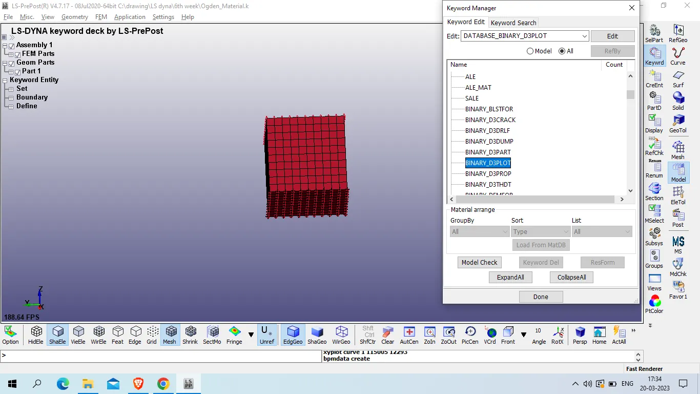
DT: 0.01

ACSII_OPTION

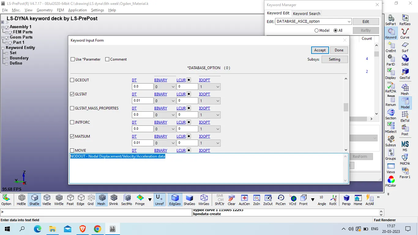
model and part >> keyword manager >> all >> database >> ASCII_OPTION

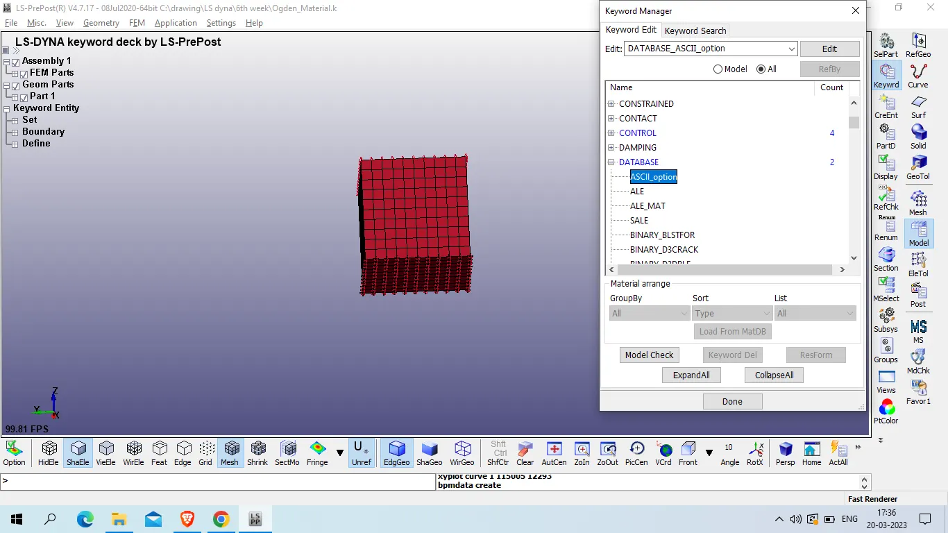
ELOUT - Element Output Data

GLSTAT - Global Statistics

MATSUM - Material Energies

NODOUT - Nodal Displacement/Velocity/Acceleration data

DT : 0.01

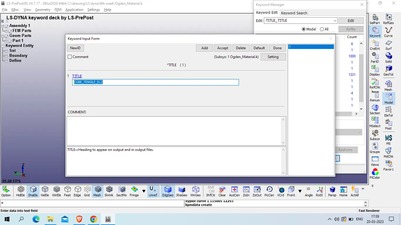
CHange the title from title card

model and part >> keyword manager >> model >> title

TITLE : CUBE_TENSILE_EL2

Acce >> done

now check for keyword error

go to model checking >> Keyword check

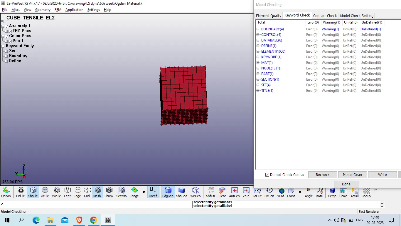
Recheck

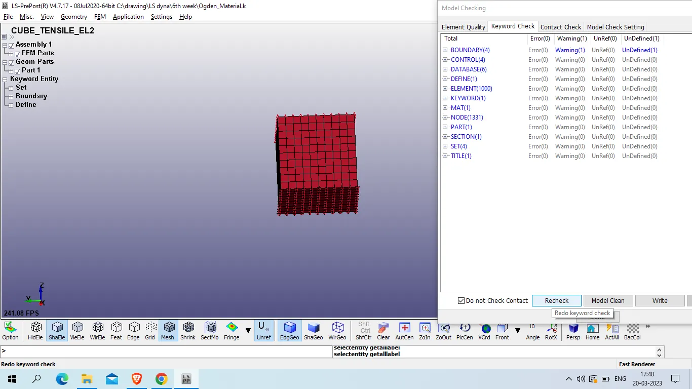
as we have zero keyword error now w'll save the model in diffrenet folder

file >> saveas >> save active keyword as

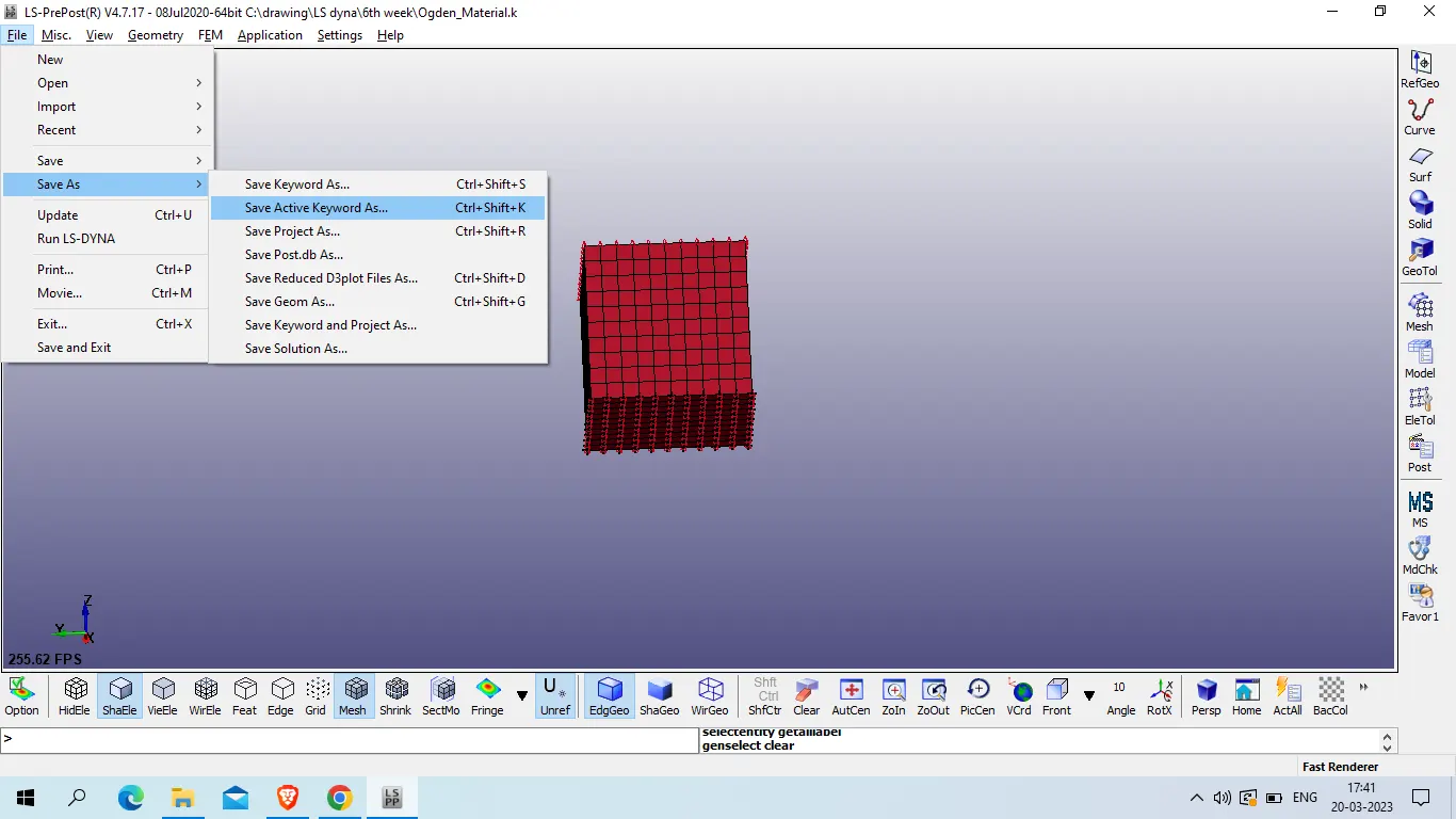
select the folder and save

after this we will run the model

file >> run LS_DYNA

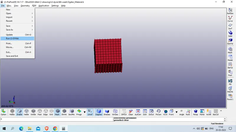
now select the file and run

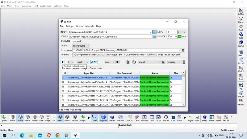
our simulation was normal terninated

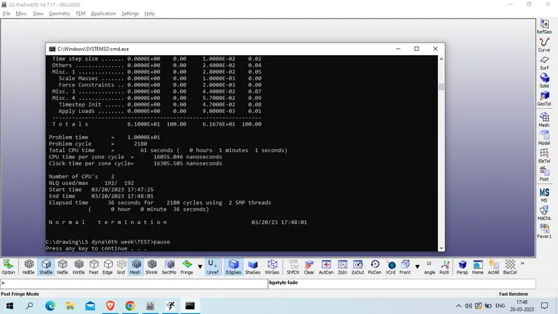
for other cases we will change the element formulation in section>> solid and run on same setting

ELFORM : 1 : constant stress solid element (default),
underintegrated constant stress ; needs hourglass stabilisation; efficient and accurate

ELFORM : 2 : fully integrated S/R solid,
Reduced integrated ; no hour glass stabilisation needed; slower than ELFORM 1; shear locking can occur

ELFROM : -1 : fully integrated S/R solid intended for elements with poor aspect ratio, efficient formulation.
Similiar to ELFORM 2 , but shearlocking is accounted for; efficient formulation (CPU time)

ELFORM : -2 : fully integrated S/R solid intended for elements with poor aspect ratio, accurate formulation.
Similiar to -1 , more accurate, more computational cost.

Result

Von mises stress in case 1 : ELFORM 1

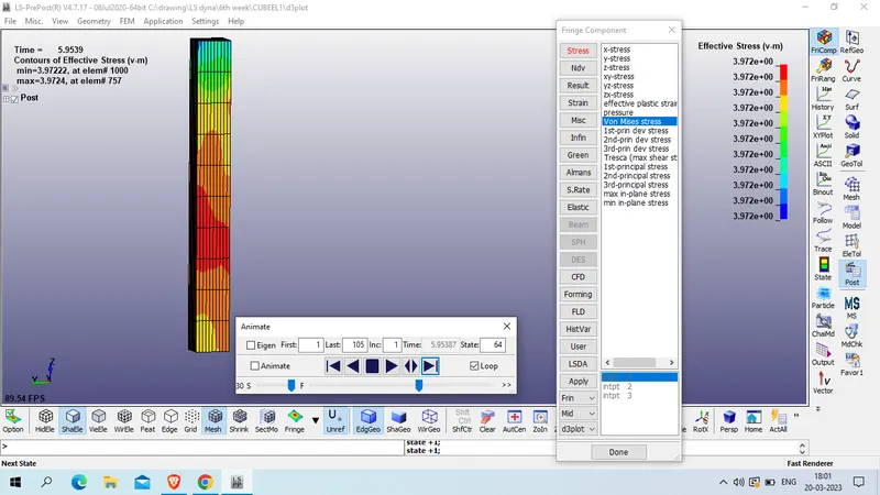
VOn Mises Stress in case 2: ELFORM 2

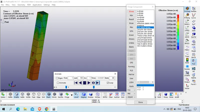
VOn Mises stress In case 3: elform -1

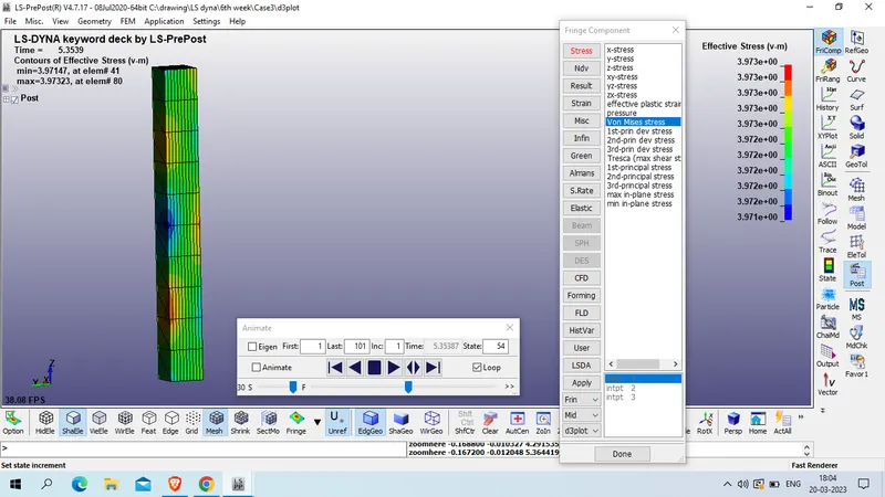
Von Mises Stress in case 4: ELFORM -2

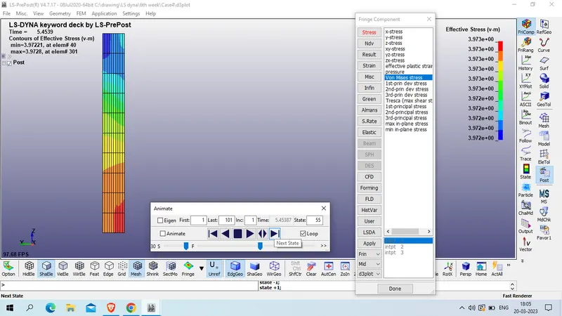
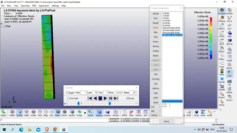
VOn Mises Strain in case 1 : ELFORM 1

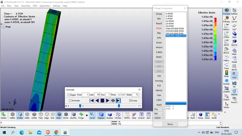
VOn mises strain in case 2: elform 2

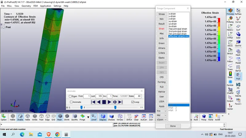
VOn Mises strain in case 3 :ELFORM -1

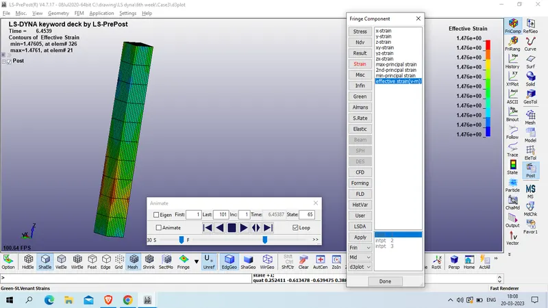
VOn Mises Strain In case 4 :ELFORM -2

Stress plot In z azis at element no 751 in case 1.

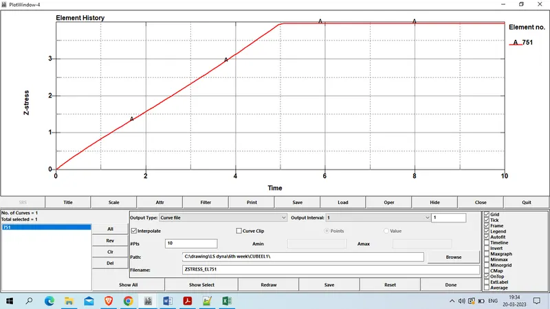
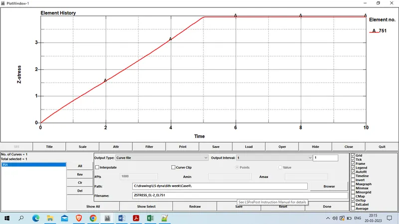
Stress plot In z azis at element no 751 in case 2.

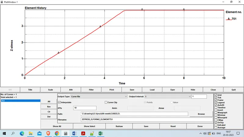
Stress plot In z azis at element no 751 in case 3.

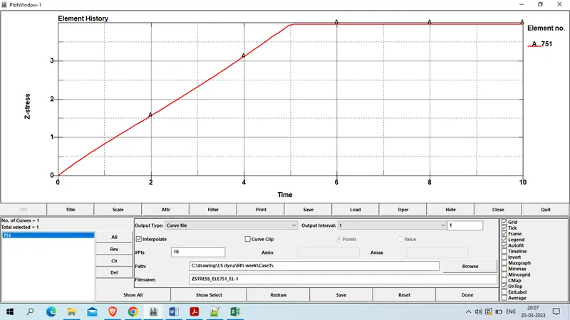
Stress plot In z azis at element no 751 in case 4.

STrain plot in z axis at element no 751 in case 1.

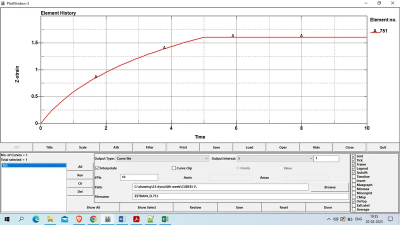
Strain plot in z axis at element no 751 in case 2.

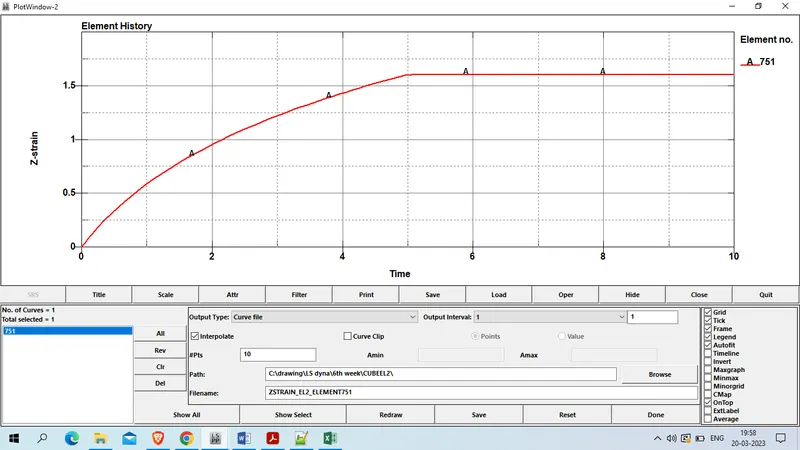
Strain plot in z axis at element no 751 in case 3.

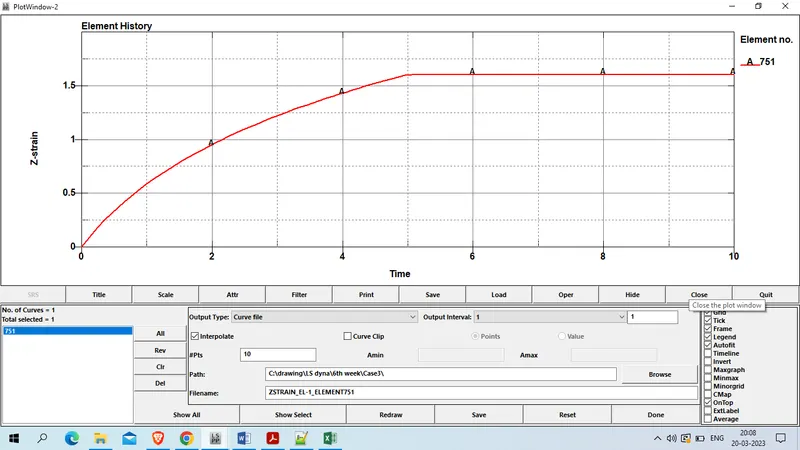
Strain plot in z axis at element no 751 in case 4.

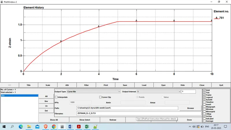
Case 1 : ELFORM 1

True Stress Vs True strain plot at element no 751 in case 1.

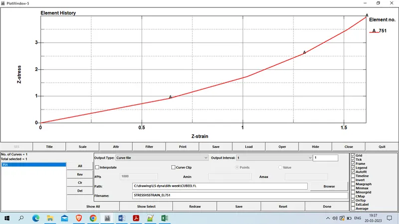
True Stress Vs True strain plot at element no 751 in case 2.

True Stress Vs True strain plot at element no 751 in case 3.

True Stress Vs True strain plot at element no 751 in case 4

Now we will calculte the engineering strain and engineering stress with below formula.

we know that ,

True strain

Ɛ_t = ln (1 + Ɛ_e)

So that ,

Ɛ_e = e^(Ɛt) -1

where, Ɛ_t = True Strain and Ɛ_e = ENgineering strain

and for true stress we have

True stress formula

σ_{t =} σ_e (1+ Ɛ_e)

so that ,

σ_e= σ_t / ( (1+ Ɛ_e)

where, σ_t = True stress and σ_e= ENgineering stress.

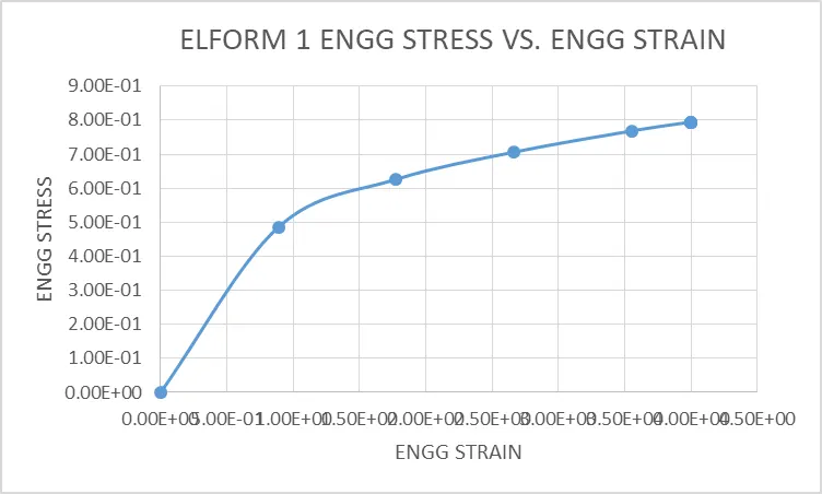
from above grapg we have data of true stress and true strain , so that we had calculated engineering strain and engineeing stress values as below

True Strain	True Stres	engg strain	engg stress
0.00E+00	0.00E+00	0.00E+00	0.00E+00
6.36E-01	9.17E-01	8.88E-01	4.85E-01
1.02E+00	1.74E+00	1.78E+00	6.26E-01
1.30E+00	2.59E+00	2.67E+00	7.06E-01
1.52E+00	3.50E+00	3.55E+00	7.69E-01
1.61E+00	3.97E+00	4.00E+00	7.95E-01
1.61E+00	3.97E+00	4.00E+00	7.95E-01
1.61E+00	3.97E+00	4.00E+00	7.95E-01
1.61E+00	3.97E+00	4.00E+00	7.95E-01
1.61E+00	3.97E+00	4.00E+00	7.95E-01

Graph for engineeing stress and engineering strain as given below

Case 2 : ELFORM 2

True Stress Vs True strain plot at element no 751 in case 2.

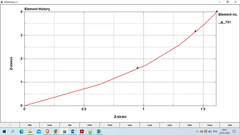
from above grapg we have data of true stress and true strain , so that we had calculated engineering strain and engineeing stress values as below

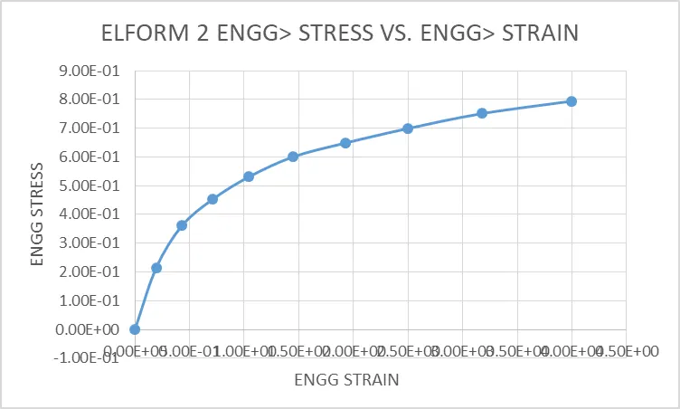
True Strain	True Stres	engg strain	engg stress
0.00E+00	-2.37E-16	0.00E+00	-2.37E-16
1.79E-01	2.58E-01	1.96E-01	2.16E-01
3.58E-01	5.16E-01	4.30E-01	3.61E-01
5.36E-01	7.74E-01	7.10E-01	4.52E-01
7.15E-01	1.09E+00	1.04E+00	5.31E-01
8.94E-01	1.47E+00	1.45E+00	6.00E-01
1.07E+00	1.90E+00	1.92E+00	6.49E-01
1.25E+00	2.44E+00	2.50E+00	6.99E-01
1.43E+00	3.14E+00	3.18E+00	7.51E-01
1.61E+00	3.97E+00	4.00E+00	7.95E-01

Graph for engineeing stress and engineering strain as given below for case 2

for case 3: ELFORM -1

True Stress Vs True strain plot at element no 751 in case 3.

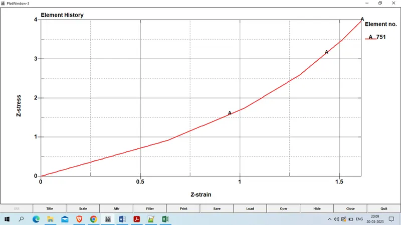
from above grapg we have data of true stress and true strain , so that we had calculated engineering strain and engineeing stress values as below

True Strain	True Stres	engg strain	engg stress
0.00E+00	-2.23E-16	0.00E+00	-2.23E-16
1.79E-01	2.58E-01	1.96E-01	2.16E-01
3.58E-01	5.16E-01	4.30E-01	3.61E-01
5.36E-01	7.74E-01	7.10E-01	4.52E-01
7.15E-01	1.09E+00	1.04E+00	5.31E-01
8.94E-01	1.47E+00	1.44E+00	6.00E-01
1.07E+00	1.90E+00	1.92E+00	6.49E-01
1.25E+00	2.44E+00	2.50E+00	6.99E-01
1.43E+00	3.14E+00	3.18E+00	7.51E-01
1.61E+00	3.97E+00	4.00E+00	7.95E-01

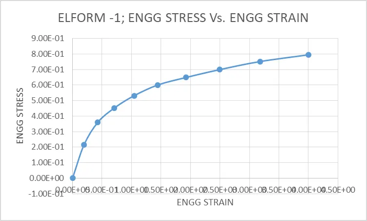
Graph for engineeing stress and engineering strain as given below for case 3

case 4: ELFORM -2.

True Stress Vs True strain plot at element no 751 in case 4.

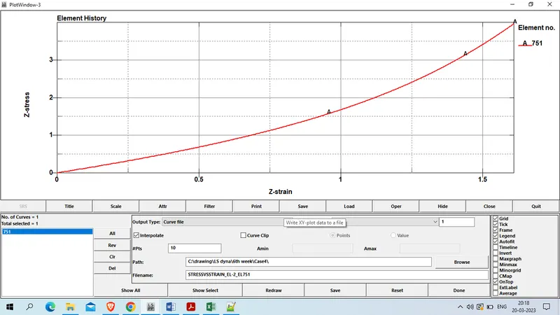
from above grapg we have data of true stress and true strain , so that we had calculated engineering strain and engineeing stress values as below

True Strain	True Stres	engg strain	engg stress
0.00E+00	-1.09E-15	0.00E+00	-1.09E-15
1.79E-01	2.24E-01	1.96E-01	1.88E-01
3.58E-01	4.71E-01	4.30E-01	3.29E-01
5.36E-01	7.47E-01	7.10E-01	4.37E-01
7.15E-01	1.06E+00	1.04E+00	5.20E-01
8.94E-01	1.43E+00	1.45E+00	5.86E-01
1.07E+00	1.88E+00	1.92E+00	6.42E-01
1.25E+00	2.42E+00	2.50E+00	6.93E-01
1.43E+00	3.11E+00	3.18E+00	7.44E-01
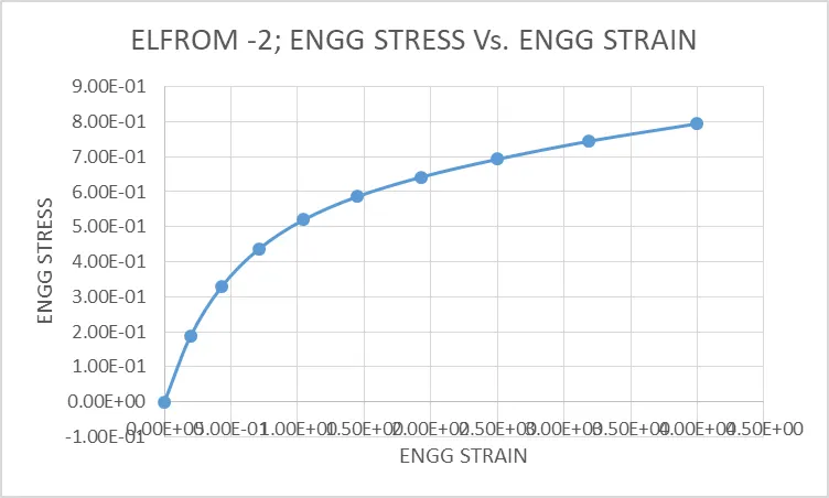
1.61E+00	3.97E+00	4.00E+00	7.95E-01

Graph for engineeing stress and engineering strain as given below for case 4

COnclusion :

There is no much difference in values of stresses between the formulation for stretch of 5.

Usage of different element formulation depends on accuracy or effiency (cpu time) requirements. In this case a large variation could not be found, when model is large enough we can notice a significant difference in the computation time.