Calculation of the Stretch Ratio by comparing the ELFORM (-2,-1,1,2) with Ogden_Material Model in LS-Dyna

Objective: Calculate the Stretch Ratio by comparing the ELFORM (-2,-1,1,2) with Ogden_Material Model.

Procedure:

• Open the provided file in the LS-Prepost. It contains the material card data.
• Navigate to the Shape Mesher option in the Mesh menu in the right ribbon.

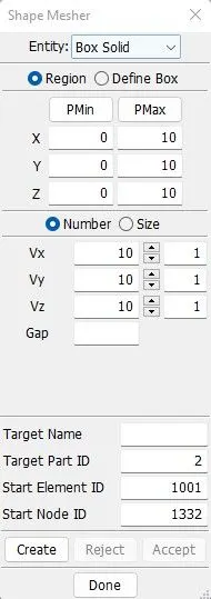
Fig 1: Options for creating a box solid.

• Enter the show values above to create a box solid with ten elements in XYZ's direction.

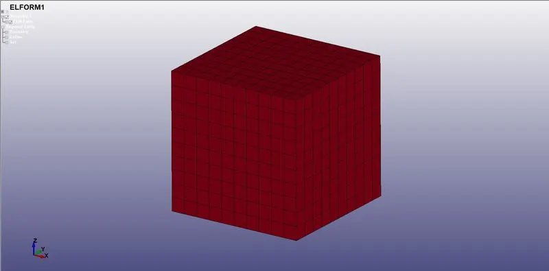
Fig 2: A solid box with 10mmx10mmx10mm dimensions is created.

• A solid section card is created with an ELFORM =1.

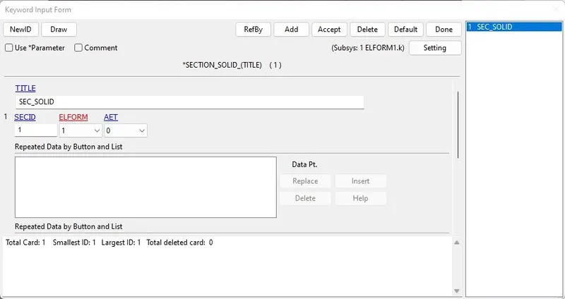
Fig 3: Solid section card is defined.

• The material card is provided, and no value is changed in the card.

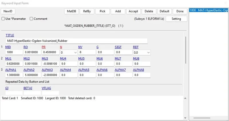
Fig 4: Material card data.

• The part is defined properly with a proper name, and the material and section are assigned to the solid box.

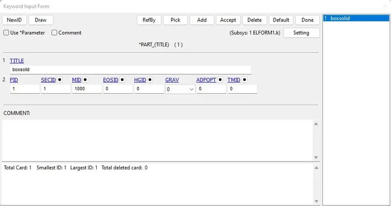
Fig 5: The part is completely defined.

• To simulate tensile behavior for the model, proper boundary conditions must be given. One side of the cube is completely constrained in the x-direction.

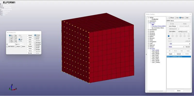
Fig 6: The side of the cube is restricted in the x-direction.

• Additionally, to add stability to the model, two more SPC are created in the lateral and longitudinal direction of the cube's face. They are constrained in y and z-direction, respectively.

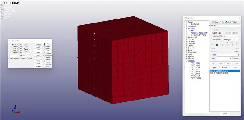
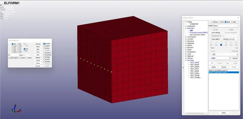
Fig 7: Two additional constraints for the stability of the solution.

• On the opposite face of this cube, displacement is provided as a Prescribed motion.

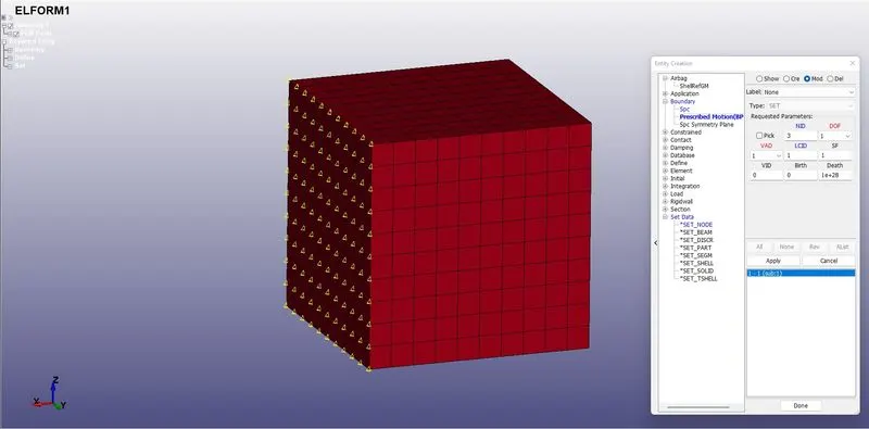
Fig 8: Displacement on the nodes of the face of the cube.

• Stretch = 1 + Engg strain

`5 =1+((Displacement)/10)`

Displacement= 40mm

• The displacement curve is defined using a curve keyword from the define deck.

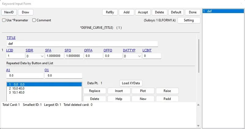
Fig 9: The displacement curve is defined.

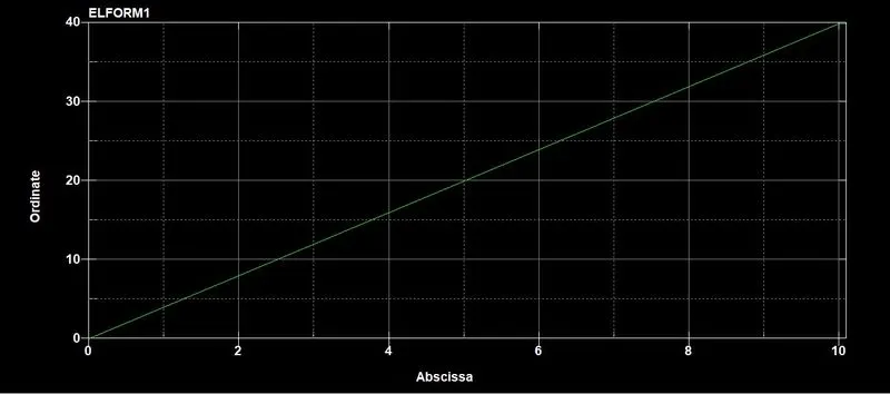
Fig 10: Displacement curve.

• To solve this particular simulation implicit solver is chosen. To define the implicit solver, specific implicit keywords must be included.
• IMPLICIT_AUTO, IMPLICIT_GENERAL, IMPLICIT_SOLUTION, and IMPLICIT_SOLVER keywords must be added from the control deck.

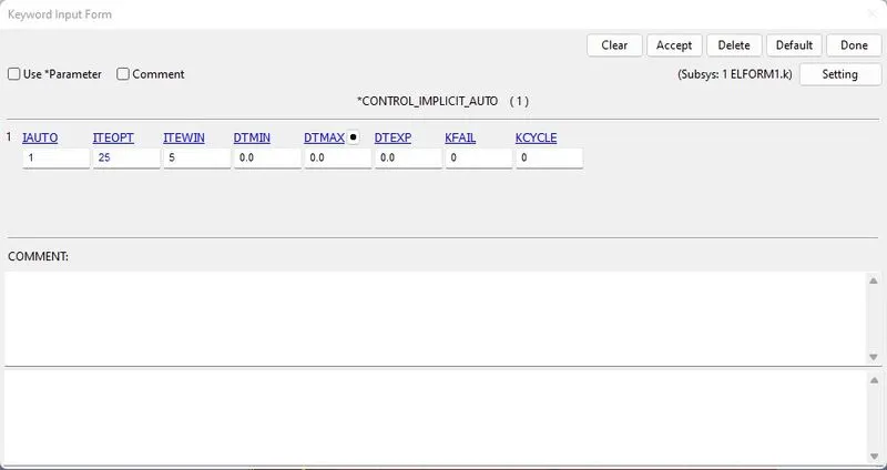
Fig 11: Implicit_auto card is defined.

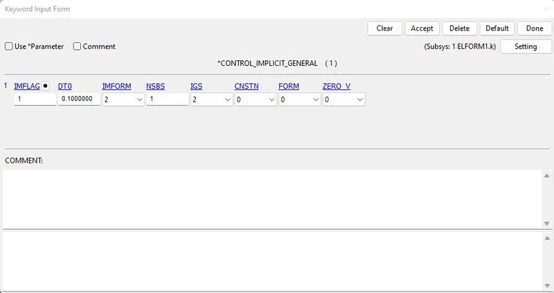
Fig 12: Implicit_general card is defined.

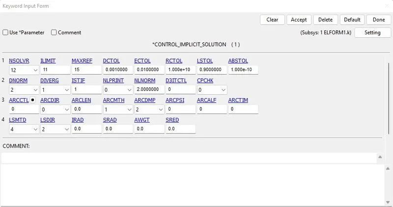
Fig 13: Implicit_solution card is defined.

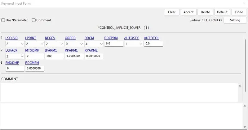
Fig 14: Implicit_solver card is defined.

• The ASCII_option keyword from the DATABASE deck is used for the output requests, and the GLSTAT option is checked.

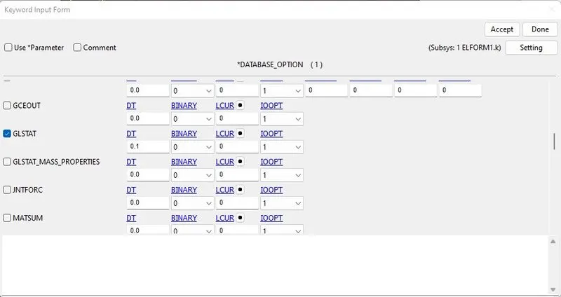
Fig 15: Output requests are defined.

• The BINARY_D3PLOT keyword from the DATABASE deck is used for the plots, and a DT of 0.1 is entered.

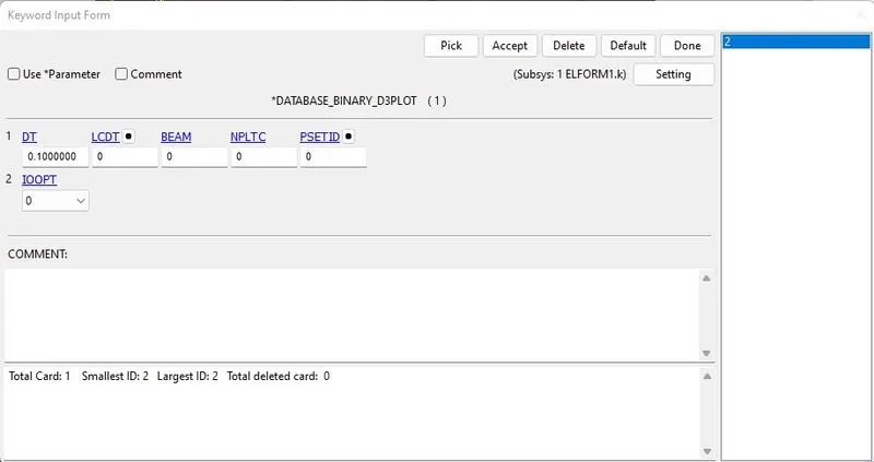
Fig 16: Plots at time intervals are defined.

• DATABASE_EXTENT_BINARY card with STRFLG =1 is used to compute the elastic strain in the model.

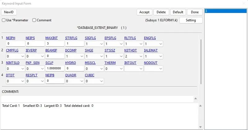
Fig 17: Elastic strain computation is enabled.

• Finally, the TERMINATION keyword from the CONTROL deck is used to define the end time of the simulation.

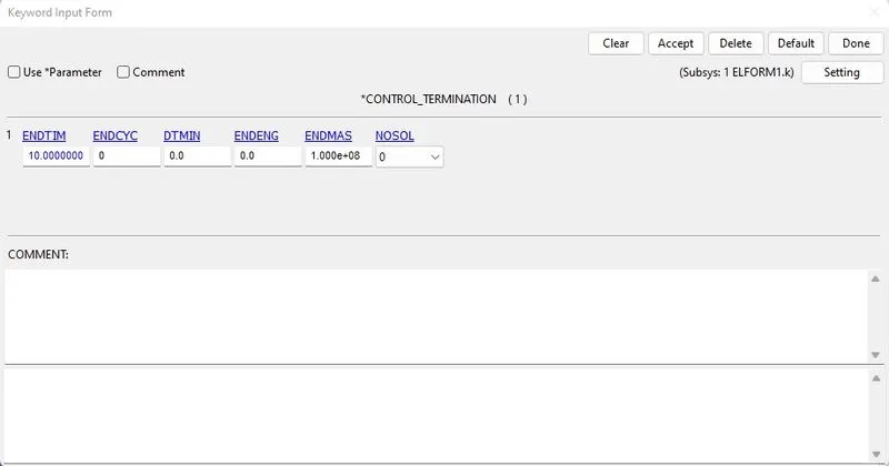
Fig 18: End time for the simulation is defined.

• With all these keywords included, the deck is fully defined and is now ready to solve.

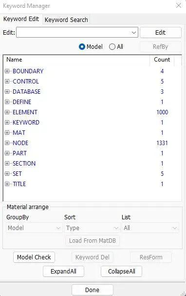
Fig 19: Fully defined deck.

• Open the Start LS-Dyna analysis, browse the keyword file, and hit run to run this keyword file.

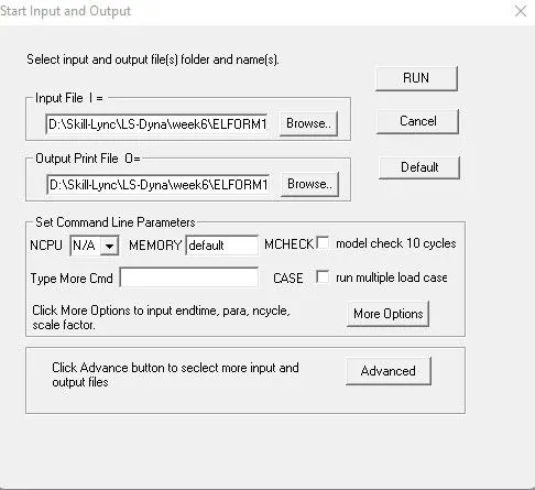
Fig 20: LS-Dyna analysis browser.

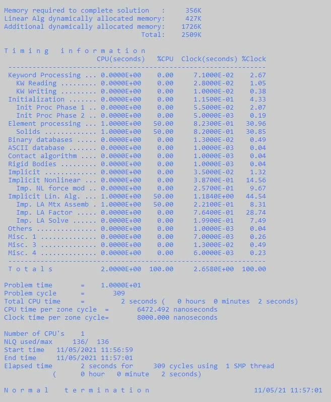
Fig 21: Successful completion of solving.

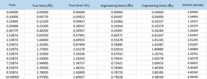
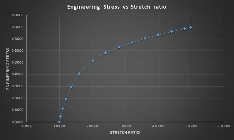
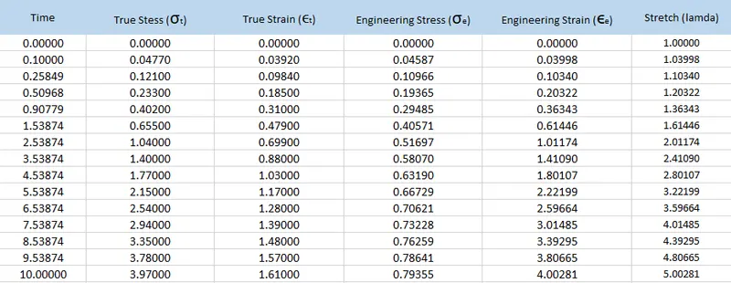
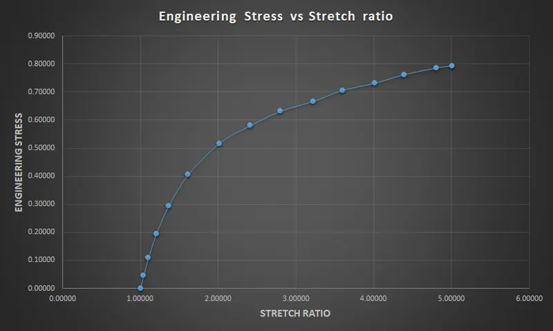
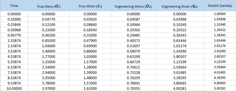
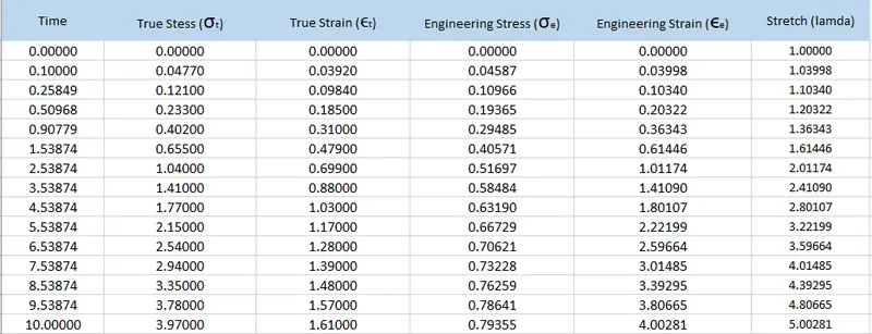
• True stress and strain curves have been plotted and saved in.csv format, and then the graphs have to be plotted for engineering stress and stretch. This is required to convert true stress and true strain to engineering stress, and strain and engineering strain are converted to stretch using these formulae.

`epsilonunderset(t) = ln(1+underset(e)(epsilon))=ln λ`

To find the engineering strain natural log when taken to the other side, the engineering strain is the (exponential of true strain - 1).

`epsilonunderset(e) = Exp(underset(t)(epsilon)) - 1`

To find stretch, one is added to engineering strain.

`lamda= 1+epsilonunderset(e)`

Finally, engineering stress is obtained by dividing the true stress with stretch.

`underset(t)(sigma) = sigmaunderset(e) * (1 + underset(e)(epsilon))`

`sigmaundersett = sigmaundersete * lamda`

`sigmaundersete = underset(t)(sigma)/ lamda`

ELFORM=1:

• Open new LS-PRE POST from the launch manager and open the LS-DYNA Binary plot (choose the D3PLOT file created) from the file menu.
• The model will be loaded the same as before, but we can access only the post-processing options from the right ribbon menu.

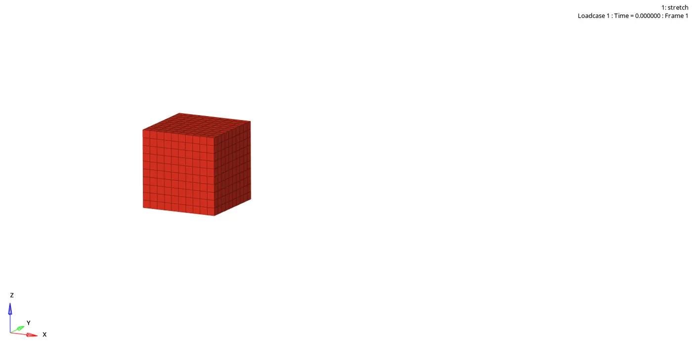
• The above animation represents the stretch in the solid block with ELFORM 1.

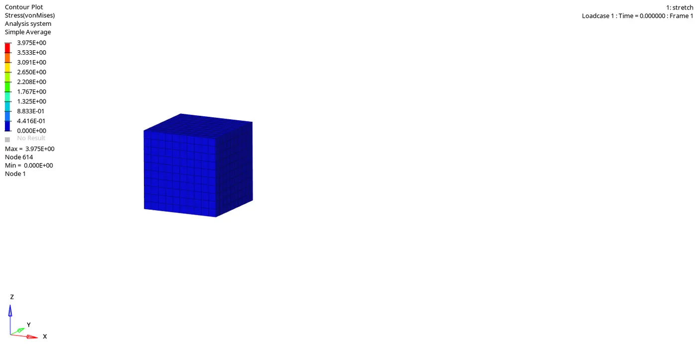
• The above animation represents the von mises stress in the solid block due to stretch with ELFORM 1.

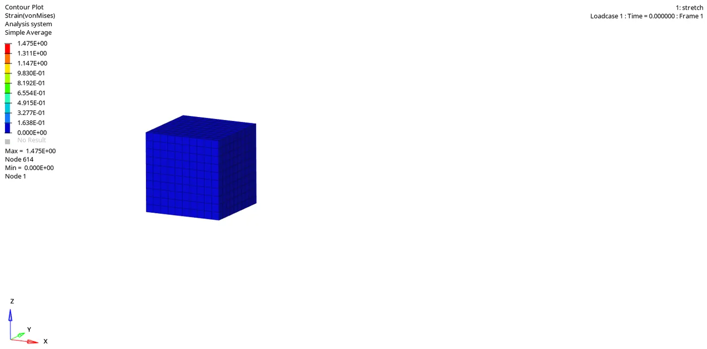
• The above animation represents the von mises strain in the solid block due to stretch with ELFORM 1.

ELFORM=2:

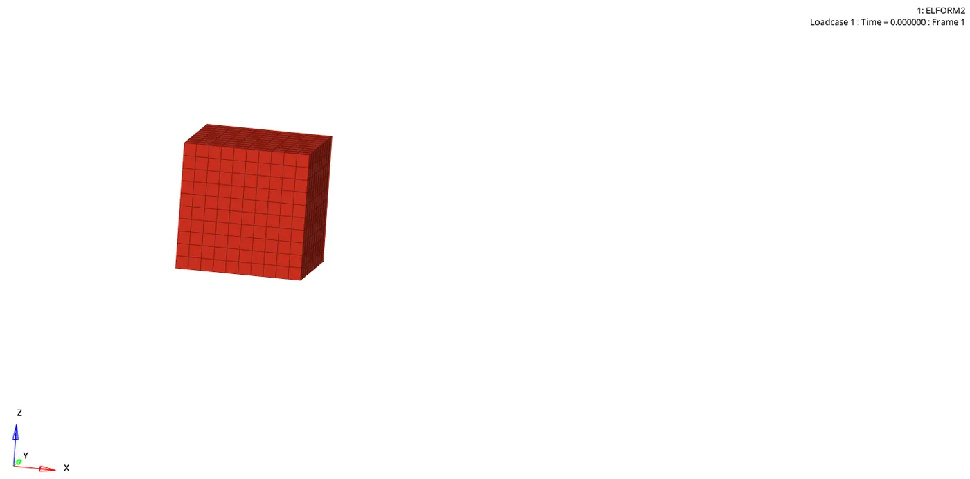
• The above animation represents the stretch in the solid block with ELFORM 2.

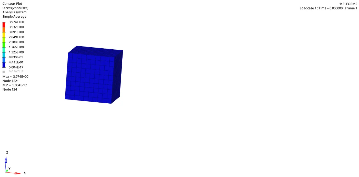
• The above animation represents the von mises stress in the solid block due to stretch with ELFORM 2.

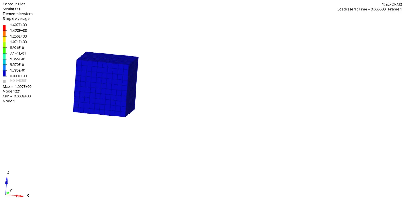
• The above animation represents the von mises strain in the solid block due to stretch with ELFORM 2.

ELFORM=-1:

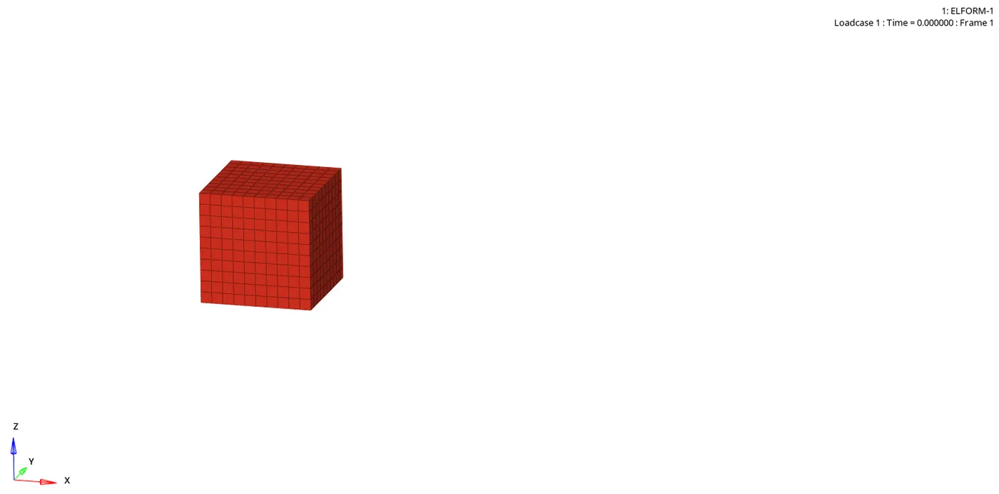
• The above animation represents the stretch in the solid block with ELFORM -1.

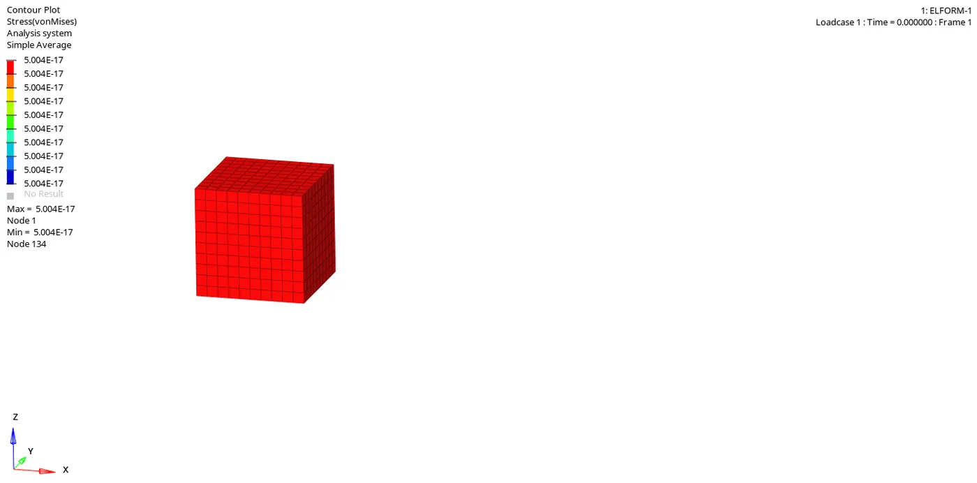
• The above animation represents the von mises stress in the solid block due to stretch with ELFORM -1.

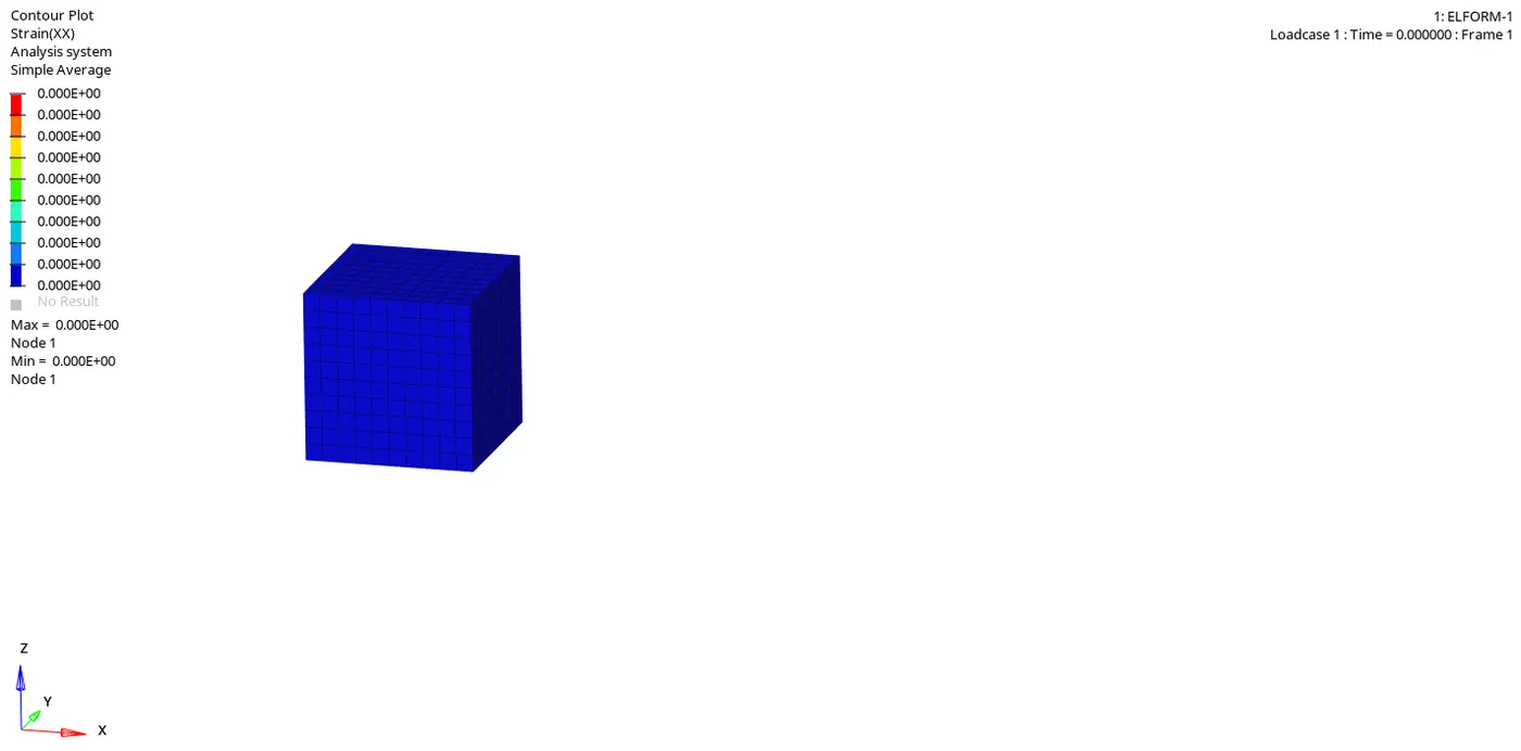
• The above animation represents the von mises strain in the solid block due to stretch with ELFORM -1.

ELFORM=-2:

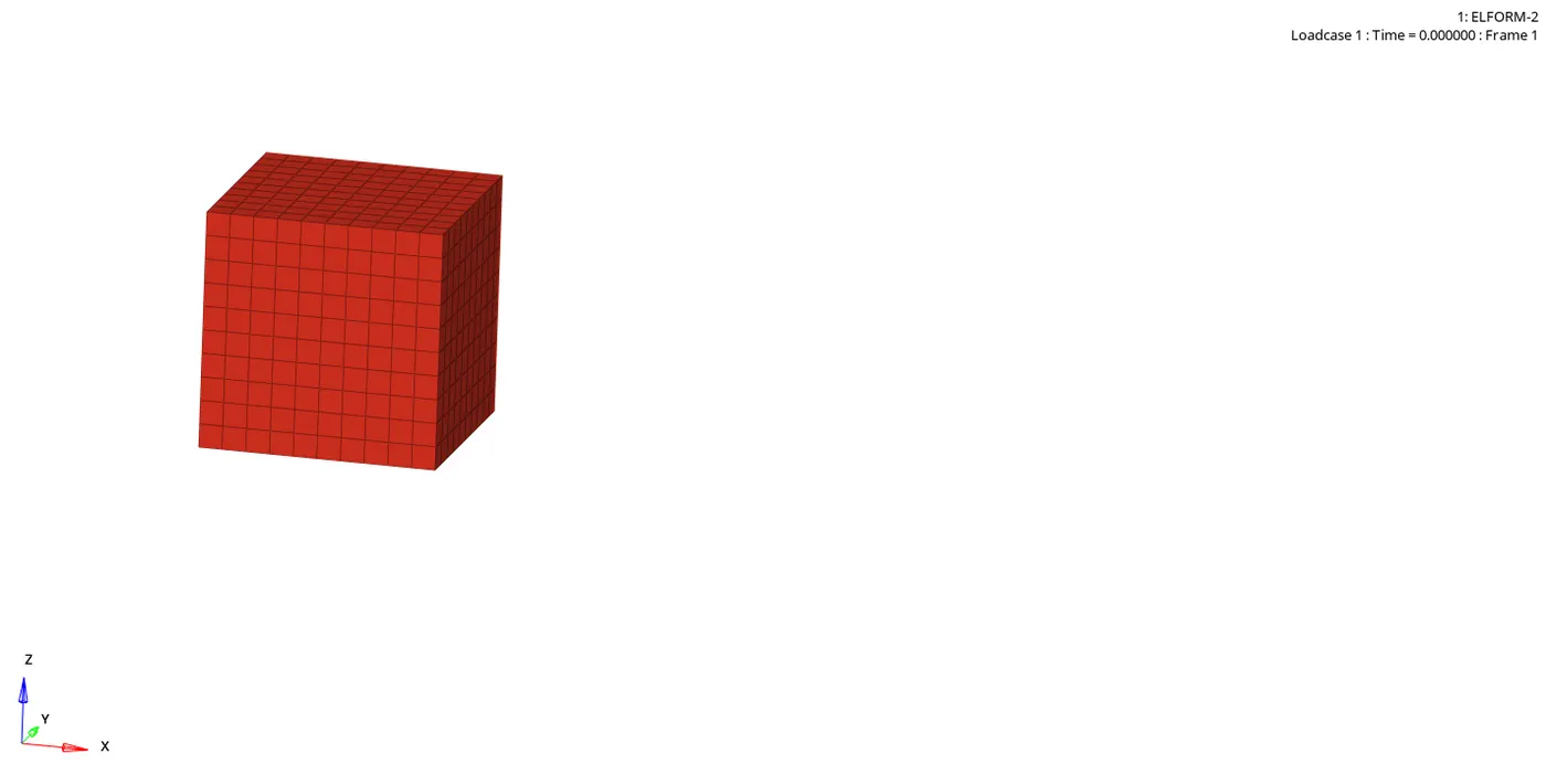
• The above animation represents the stretch in the solid block with ELFORM -2.

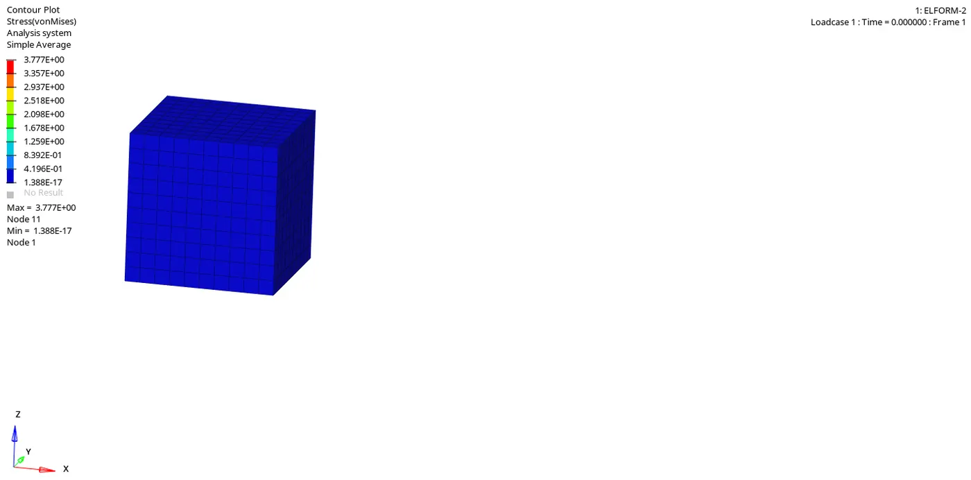
• The above animation represents the von mises stress in the solid block due to stretch with ELFORM -2.

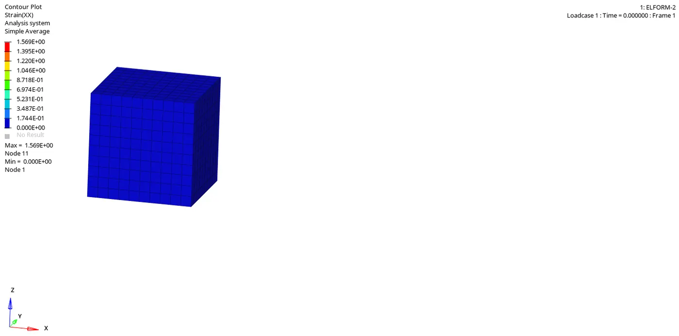
• The above animation represents the von mises strain in the solid block due to stretch with ELFORM -2.

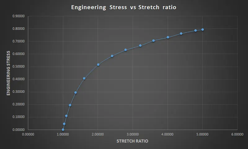
Conclusions:

• From the stretch ratio plots, it can be inferred that there is a considerable deviation from the actual plot given in the problem statement.
• The plots for various element formulations are almost the same. It is due to the simplicity of the model.
• If there is a complex geometry involved, then significant change can be observed in the results. Here, the actual test-up might not be given as the boundary conditions for the problem. For example, temperature plays a significant role during the test. Also, the rate of application of load varies in actual when compared to simulated results, thereby causing deviation in the obtained results.
• The case setup was done as per the objective, and the corresponding output requests were obtained. An implicit solver is used for the simulation because the effect of strain rates is minimal.
• The value of the stretch ratio is calculated for various element formulations.