Week 5 - Turbulence modelling challenge

Aim: To perform literature on different turbulence models used and simulate Aerodynamic simulation on the Golf Ball and post process the results.

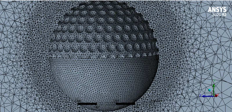
Simulation: The Golf ball that is to be simulated, is with dimples on one half and a smooth surface on the other half. In this simulation, we are interested more in the drag and lift

Type of flows:

The type of flow mostly depends on the Reynolds number

Laminar flow: when the Reynolds number is less than the critical number, the critical number varies for different geometries. Viscous forces are dominant.

Turbulent flow: when the Reynolds number is greater than the critical number (eddy, vortex formation begins). Inertial forces are dominant.

Transition flow: there is a transition from the laminar to the turbulent flow, both the inertial and viscous forces are dominant.

Laminar flows are regular and highly stable, predictable in nature but turbulent flows are highly random and unpredictable in nature. so to simulate the turbulent flows scientists averaged the disturbances into coherent structures called vortices. These help in better modeling the turbulent flows. There are many turbulent models present they are:

These models are classified in many ways one is based on the Order of the model

First Order Models:

In these models, the PDEs used to solve the turbulence are of First-order so these models are called first Order Models. This assumes an analogy between laminar and turbulent flows. Average turbulent flow field is similar to corresponding laminar flow. These models are best suited for good results with less computational power power and less cost compared to second order model. These are usually used to solve turbulent viscosity.

Zero Equation model:

In this model, no PDEs are used to solve for turbulence viscosity. It will not account for the turbulent behavior of the turbulent viscosity. Directly solves the turbulent viscosity using the mixing length model. It assumes eddy viscosity terms to be dimensionally similar to two Kolmogorov scales length scales and velocity scales.

One equation model( Spalart Allmaras model)

The Spalart–Allmaras model is a one-equation model that solves a modeled transport equation for the kinematic eddy turbulent viscosity. The Spalart–Allmaras model was designed specifically for aerospace applications involving wall-bounded flows (Internal flows). specifically when the flow is attached to the body. The Spalart-Allmaras model has been implemented to use wall functions when the mesh resolution is not sufficiently fine.

Two equation model

These models use two PDE's to solve for

• Turbulent kinetic energy and Turbulence dissipation rate
• Turbulent kinetic energy and Specific dissipation rate

The two-equation model is the most widely used in the industries.

- k-epsilon model:

This model is suitable for turbulent flows without flow separation. This model belongs to the RANS model (Reynolds averaged Navier stokes equation)

1. Standard k-epsilon:

This is the most widely used model for industrial applications because of quick results. It uses wall functions to model near the wall. These models have good convergence and require less computer memory. Very good results for the attached turbulent flows over external bodies and complex structures. the disadvantage is that its results are very bad for separating flows.

2. Realizable k-epsilon model:

This is the modified epsilon equation model. Shows some consistent results with the turbulent models. It also exhibits superior performance for flows involving rotation, boundary layers under strong adverse pressure gradients, separation, and recirculation. In virtually every measure of comparison, Realizable k-ɛ demonstrates a superior ability to capture the mean flow of the complex structures.

3. Renormalized group(RNG) k-epsilon:

It is has a much-improved epsilon equation with the modeling for the swirling effect included. It uses empirical relations to find a modified version of Prandtl Number.

- K-omega model:

This is one of the most popularly used models in the industry. This model belongs to the RANS model (Reynolds averaged Navier stokes equation)

1. Standard k-omega model:

The standard k−ω model is a low Reynolds number model, it can be used for flows with low Reynolds number where the boundary layer is relatively thick and the viscous sublayer can be resolved. Thus, the standard model is best used for near-wall treatment. Other advantages include a superior performance for complex boundary layer flows under adverse pressure gradients and separations.

2. SST k-omega model:

shear stress transport k -omega model. It is an improved version of the standard k-omega model. It models best for the near wall and the free stream. It is the most popular model when modeling near the wall and away from the wall is needed. Uses a blending function to transition from a standard model to a high Reynolds model away from the wall.

Second-Order Models:

Solves transport equations for the Reynolds stress terms. These models give the most accurate results and are highly sensitive to boundary conditions. They are also computationally expensive.

• Algebraic Stress model

algebraic Reynolds stress model is developed from the modeled dynamic equations for the Reynolds stress.

• Reynolds Stress model

RSM is more offers better accuracy in flows with high degrees of anisotropy, significant streamline curvature, flow separation, zones of recirculating flow, or flows influenced by rotational effects for which k-omega and k epsilon gives unsatisfactory results.

Kolmogrov scale of turbulence:

Smallest scales of turbulence can be estimated through advanced theoretical fluid dynamics. Cascade process of turbulence represnets transfer of turbulent kinetic energy from larger eddies to smaller eddies.

Universal equilibrium theory states that smaller eddies should recieve energy from larger eddies and dissipate that energy at nearly an equal rate into heat and accoustic radiation. The motion of small scales depends mainly on which larger eddies supply energy and kinematic viscosity is equal to

`-(dK)/(dT)`

`eta=((nu^3)/(epsilon))^(1/4`

`tau=(nu/(epsilon))^(1/2)`

`nu=(nu*epsilon)^(1/4)`

The first equation represnts the smallest length scale. The second equation represnts the time scale and the third equation represents theb velocity scale.

Most simple example is fourier decomposition of energy into wave numbers .

why DNS isn’t feasible according to Kolmogorov's scale.

The challenge in turbulence modeling is the modeling of the eddies.

• Eddy is the swirling of a fluid and the reverse current created when the fluid is in a turbulent flow regime i.e when the flow around the body exceeds critical velocity.
• Larger eddies break into smaller eddies on consuming smaller eddies and sometimes smaller eddies combine to form larger eddies This process is called energy cascading.

`size prop(L/U_oo)`

Larger eddies gain energy from the mean flow.

`size propL/(Re)^(3/4)`

Smaller eddies gain energy from large eddies

• Kolmogorov is a mathematician who developed Kolmogorov scales, Kolmogorov's theory describes how energy is transferred from larger to smaller eddies; how much energy is contained by eddies of a given size; and how much energy is dissipated by eddies of each size. Kolmogorov's length scale, time scale, and velocity scale.
• Kolmogorov's length scale is the smallest

`eta=((nu^3)/(epsilon))^(1/4`

`eta = U^3/L`

`epsi` is the rate of dissipation of turbulent kinetic viscosity

Kolmogrov time scale

`t_n = (v/epsi)^(1/2)`

To check the feasibility of the DNS

The ratio of the largest to the smallest eddies is given below

`L/eta = L/(v^(3/4))epsi^(1/4)`

`L/eta = L/(v^(3/4)).U^(3/4)/L^(1/4)`

`L/eta = (LU^(3/4))/v`

`L/eta = Re^(3/4)`

• To model the vortex they are divided into cells containing grids and this is easy for the large vortex. the same size of the grid is not useful to resolve a small vortex, for a smaller vortex we need to reduce the size of the grid.
• The challenge always is to model the smaller vortex as the grid size is reduced the number of the grids will increase which in turn increase the computational costs.
• This leads to a very large number of 3D elements which demands more computational power and computational time. So DNS is mostly avoided but still performed in 2D simulations for some scientific applications. The usage of DNS in industrial applications impossible keeping in mind the complexities of the design and the size of the domains present.

To understand Golf Ball Dynamics, we need to know the lift and drag forces.

• when a body is moving in the air it experiences drag force and lift. Drag force is in the opposite direction to the body's relative motion, and the lift is a total upward force on the body.
• Drag is divided into pressure and friction drag, pressure drag is due to the pressure difference between the front and back of the body. The friction drag is due to the surface friction (due to no-slip near the surface there will be boundary layer formation with a gradient of velocity).
• Pressure Drag is significant in bluff bodies like spheres and friction drag is more significant in streamlined bodies.
• So more streamlining also increases friction drag.
• In history, golf balls were made with smooth surfaces and they didn't travel much farther distances like now. They observed that the more used golf balls traveling longer distances than the new ones. It didn't take long to know the reason behind it is due to the rough surface created.
• After that discovery, the golf balls were made with some irregularities later were made into dimples.
• For a smooth ball, the flow separation takes place after 80 deg in laminar flow and the turbulent flow separation is after 120 deg. The later the flow separation the lesser will be the pressure drag. we can make the flow turbulent by introducing dimples on the surface of the ball.
• The turbulent flow increases the mixing or interchanging of energy in the boundary layer, which helps the flow to be attached for the delay of flow separation.
• Once the dynamics of cricket ball were in the big picture due to the impossible inward swing, This happens because Air moves slowly over the rough side of the ball (high pressure) and quickly over the shiny side (low pressure), making an air pressure difference that causes the net force to push the ball towards the rough side.

Simulation steps:

• Import the geometry model and create the enclosure.
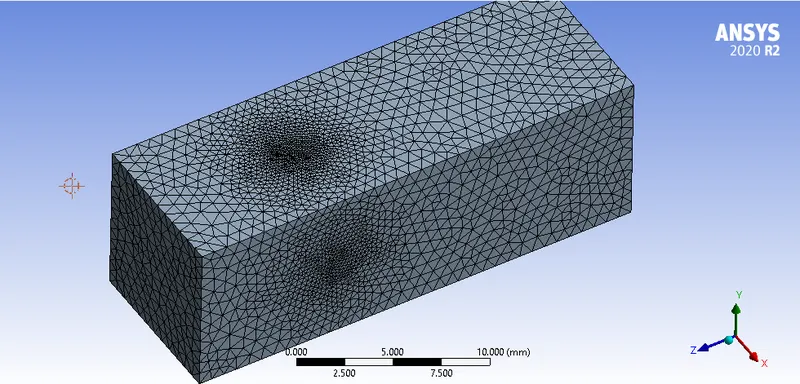
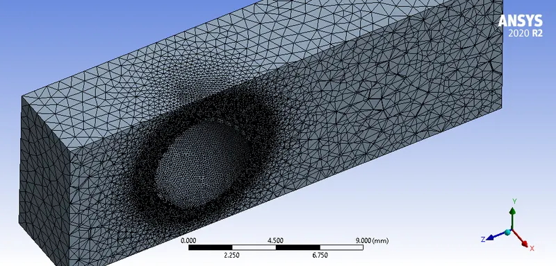
• Meshing is performed with the proper sizing and element size and see that the number of elements to be less than 5 lakh. Naming is done with inlet, outlet, and symmetry to the other walls.
• Then solver setup is done by giving the boundary conditions and the solver is selected as k-w SST. This model gives better results for near-wall and far away from the wall.
• For viewing the results in proper planes are created and plots for pressure and velocity are created.

Golf ball simulation:

- Mesh:

Golf ball simulations results:

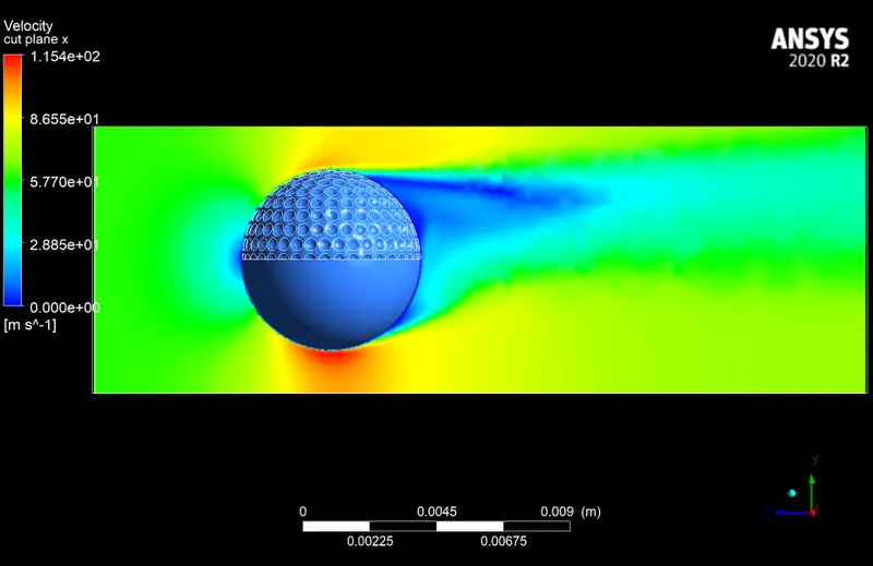
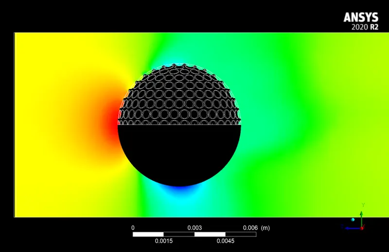
- Velocity and pressure contours:

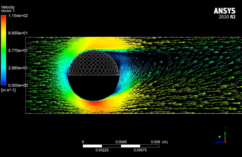
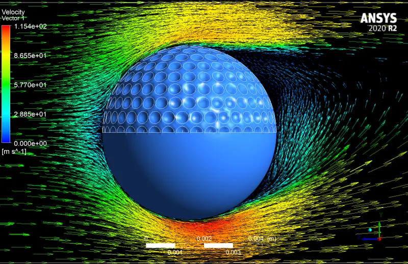
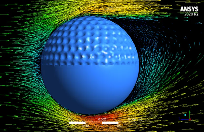
- Velocity vectors:

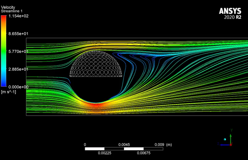
- Streamlines:

Conclusion:

The velocity of the flow below the golf ball is high so the pressure is low and a wake is created after the rough surface. The velocity of the air on the rough surface is less and the velocity of air on the smooth surface is high. This creates a difference in pressure and accounts for the swing of the ball downwards.