Week 5 - Turbulence modelling challenge

Aim: A study on Turbulence modelling, Wake region of Gulf ball using CFD simulation

Objectives:

1. To review various turbulence models and explain why DNS isn’t feasible according to Kolmogorov's scale.
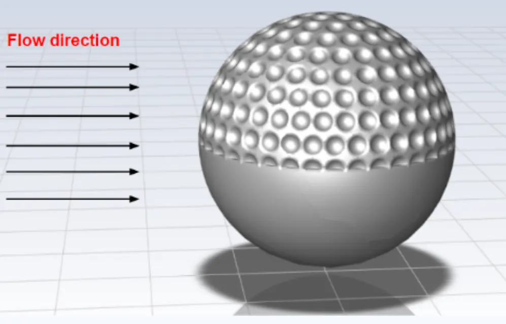
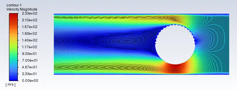
2. To perform a 3D simulation and to explain the recirculation region using velocity vectors. Consider the flow direction of air, the ball is traveling opposite to it at 60m/s. To explain in which direction the ball will curve by visualizing the wake region.

Theory:

The Reynolds number primarily determines the type of flow.

Laminar flow: Laminar flow happens when the Reynolds number is less than the critical number. The critical number varies with the different geometries. The prevailing powers are ferocious.

Turbulent flow: When the Reynolds number is beyond the critical value, an eddy or vortex begins to develop. The strongest forces are those of inertia.

Transition flow: When the flow changes from laminar to turbulent, the inertial and viscous forces become more pronounced.

Laminar flows are exceedingly steady, regular, and predictable, while turbulent fluxes are highly chaotic and unpredictable. To depict turbulent flows, scientists averaged the disturbances into coherent structures known as vortices. These help to simulate turbulent flows more accurately. There are several

First-Order Models: Because the PDEs used to solve the turbulence in these models are of the first order, they are referred to as first-order models. This presupposes that laminar and turbulent flows are analogous. In comparison to second-order models, the average turbulent flow field is comparable to equivalent laminar flow. These models are best suited for satisfactory results with less processing power and less expense. These are commonly employed to tackle problems with turbulent viscosity.

Zero Equation model: The zero equation model does not employ PDEs to account for turbulent viscosity. The turbulent behavior of the turbulent viscosity will not be taken into consideration. The mixing length model is used to solve the turbulent viscosity directly. Eddy viscosity terms are assumed to be dimensionally equivalent to two Kolmogorov scales: length scales and velocity scales.

One equation model ( Spalart Allmaras model): A model with only one equation ( Spalart Allmaras model) The Spalart-Allmaras model is a one-equation model for kinematic eddy turbulent viscosity that solves a modeled transport equation. The Spalart-Allmaras model was created with wall-bounded flows (Internal flows) in mind, especially when the flow is linked to the body. When the mesh resolution isn't fine enough, the Spalart-Allmaras model is used to generate wall functions.

Two widely used equation Models :

1. Turbulent kinetic energy and Turbulence dissipation rate
2. Turbulent kinetic energy and Specific dissipation rate are solved using two PDEs in these models.

In the industries, the two-equation model is the most often utilized.

• K-Epsilon model: The K-epsilon model is good for turbulent flows with no flow separation. The RANS model includes this model (Reynolds averaged Navier-Stokes equation)

1. Standard k-epsilon: Because of its speed, this is the most extensively used model for industrial applications. To model near the wall, it employs wall functions. These models are more convergent and use less memory on the computer. The associated turbulent flows over external bodies and complicated structures produced excellent results. The downside is that it produces poor outcomes when it comes to dividing flows.
2. Realizable k-epsilon model: The modified epsilon equation model is a realizable k-epsilon model. It also shows higher performance for flows including rotation, and boundary layers under significant unfavourable pressure gradients, separation, and recirculation when compared to turbulent models. In almost every comparison, Realizable k-€ outperforms the competition in terms of capturing the mean flow of complicated structures.
3. Renormalized group(RNG) k-epsilon: It features a much-enhanced epsilon equation that includes whirling effect modelling. It finds a modified version of the Prandtl Number using empirical relations.

• K-omega model: The K-omega model is one of the most widely utilized in the business. The RANS model includes this model (Reynolds averaged Navier stokes equation)

1. Standard k-omega model: The standard model is a low model that may be employed for low Reynolds number flows with a relatively thick boundary layer and a viscous sublayer that can be resolved. As a result, for near-wall treatment, the conventional model is optimal. Improved performance for complicated boundary layer flows under unfavourable pressure gradients and separations is another benefit.
2. SST k-omega model: Shear stress transfer k-omega model (SST k-omega model). It's a better variant of the traditional K-omega model. It's the most common model for modelling near the wall and away from the wall, and it's the most popular model for modelling near the wall and away from the wall. Transitions from a standard model to a high Reynolds model away from the wall using a mixing technique.

Second-Order Models:

Solves transport equations for Reynolds stress terms using second-order models. These models are the most precise and are most sensitive to boundary conditions. They're also time-consuming to compute.

• Algebraic Stress Model: The algebraic Reynolds stress model is derived from the Reynolds stress dynamic equations.
• Reynolds Stress model: In inflows with high degrees of anisotropy, considerable streamline curvature, flow separation, zones of recirculating flow, or flows impacted by rotational forces, the Reynolds Stress model RM provides superior accuracy than k-omega and k epsilon.
• Turbulence on the Kolmogorov scale: Advanced theoretical fluid dynamics may be used to determine the smallest sizes of turbulence. Turbulent kinetic energy is transferred from bigger eddies to smaller eddies in the cascade process.

According to universal equilibrium theory, smaller eddies should absorb energy from bigger eddies and disperse it in about equal amounts as heat and acoustic radiation. Small scale motion is mostly determined by which bigger eddies provide energy, and The smallest length scale is represented by the first equation. The time scale is represented by the second equation, while the velocity scale is represented by the third equation. The most simple example is the Fourier decomposition of energy into wavenumbers.

According to Kolmogorov's scale, DNS isn't viable.

• When a fluid is in a turbulent flow regime, i.e., when the flow around the body surpasses critical velocity, bigger eddies break into smaller eddies, and sometimes smaller eddies combine to form larger eddies. Energy cascading is the term for this process.
• We can't utilize DNS since it creates a very small mesh and tries to capture all anomalies (cells), therefore, as the number of mesh cells grows, the time it takes to solve grows. As a result, industries dislike this strategy.

The mean flow provides energy to larger eddies.

Large eddies provide energy to smaller eddies.

• Kolmogorov's theory outlines how energy is transmitted from bigger to smaller eddies, how much energy is held by eddies of a given size, and how much energy is released by eddies of each size.
• Kolmogorov's length scale is the smallest, followed by his time scale and velocity scale.

Procedure:

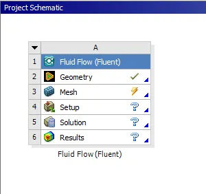
1. Open the Ansys workbench and pull Fluid Flow (Fluent) in the project schematic.
2. Import the given geometry, generate the fluid region, and make name selections for fluent input data.
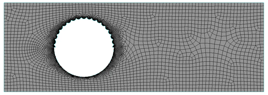
3. Generate mesh and specify Inlet, outlet & Wall faces. also the gulf ball surfaces.
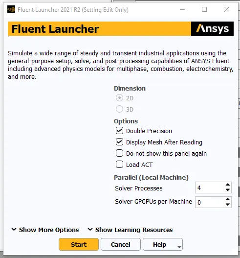
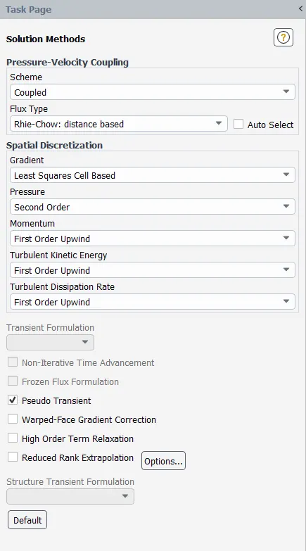
4. The start of Ansys fluent with a pressure-based solver in a steady state.
5. From the model, select 2 equations: k-epsilon, realizable, and the standard wall function.
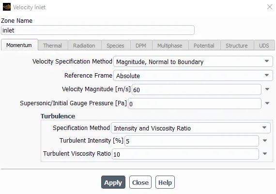
6. Input 60 m/s (given data) of Gulf ball speed in the inlet zone.
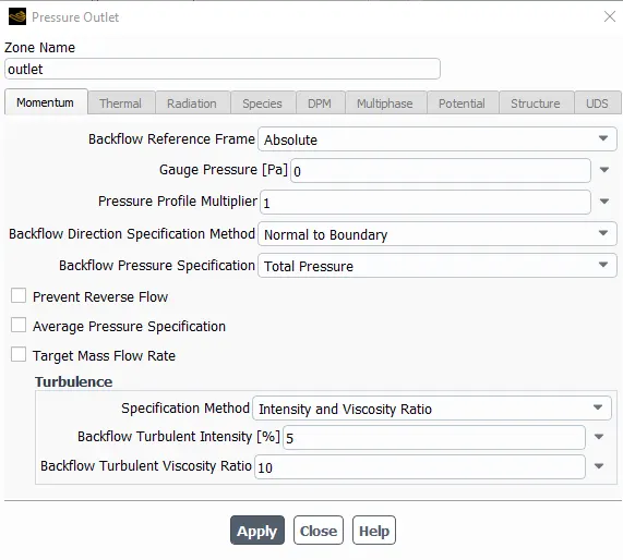
7. Output is the default, pressure in the outlet zone.
8. Material: air.
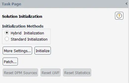
9. Initialization.
10. Run the simulation.

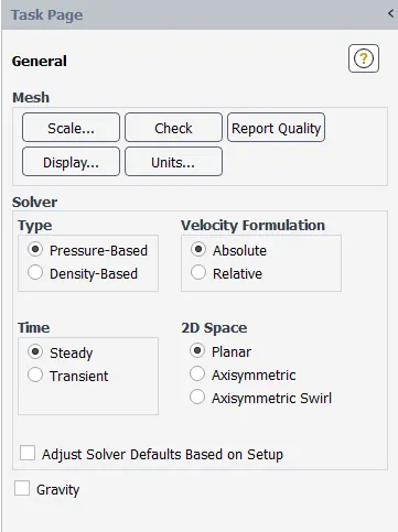
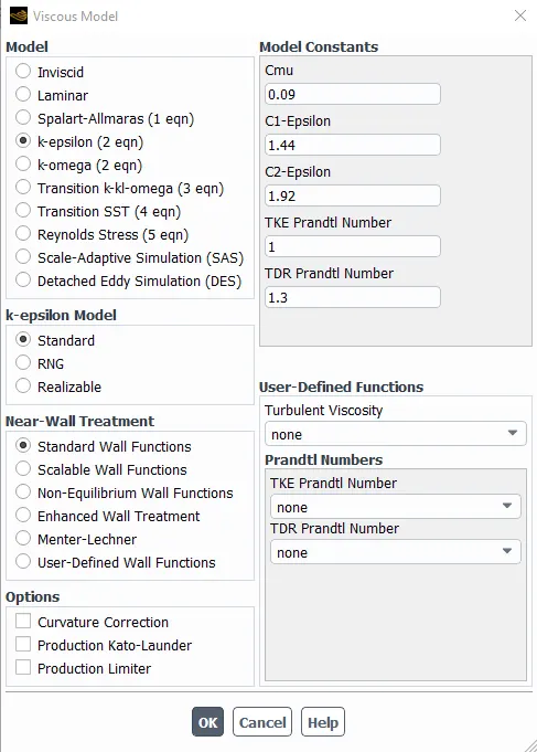
Inlet and Outlet parameters

Results:

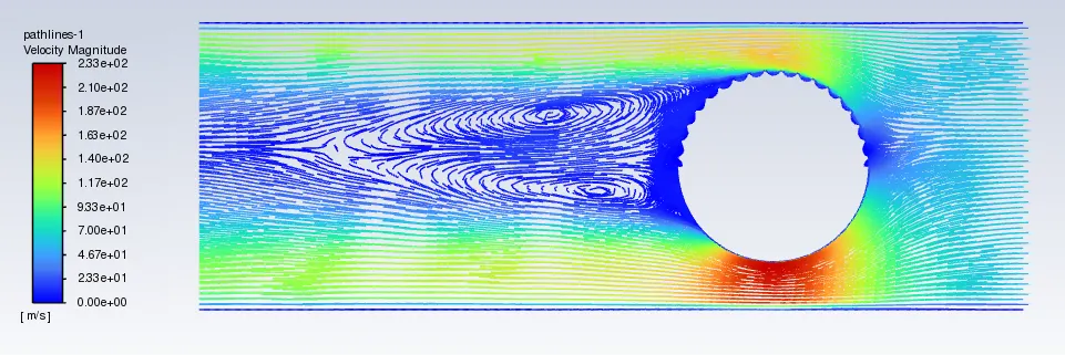
Conclusion:

1. The recirculation region is behind the ball as you can see in the streamline and vector plot of velocity magnitude.

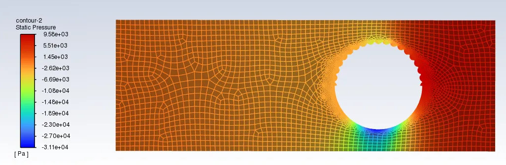
2. The gulf ball tends to move towards a downward direction because of the presence of dimples in the upper half of the ball.

3. Pressure of the upper half is more when compared to the lower half as seen in the static pressure plot.

References:

https://cfd.spbstu.ru/agarbaruk/doc/2006_Wilcox_Turbulence-modeling-for-CFD.pdf

https://www.cfd-online.com/W/images/3/31/Turbulence_Modeling_For_Beginners.pdf