Week 5 - Turbulence modelling challenge
literature
K-epsilon Model:
This model is essentially a high Reynolds number model, meaning the law of the wall must be employed and provide velocity “boundary conditions” away from solid boundaries (what is termed “wall-functions”). Another major drawback is the model's lack of sensitivity to adverse pressure-gradient. It was observed that under such conditions it overestimates the shear stress and by that delays separation.
This model is usually used where flow does not demand to integrate the solution through the viscous sublayer and wall-bounded effects are secondary. For such cases, the first cell away from the wall shall be placed at a y+ of 30-300. In such a scenario, the viscous sublayer and buffer layer (viscosity-affected inner region) are not resolved. Instead, semi-empirical formulas called “wall functions” are used to bridge the viscosity-affected region between the wall and the fully-turbulent region.
K-omega Model:
This model is essentially a low Reynolds number model. This model takes 'elliptic' near-wall behavior meaning that it has an inherent nature of being able to “communicate” with the wall and actually has Dirichlet (as in no-slip in this case) boundary conditions. The implication of such behavior is the straightforward possibility of integrating through the laminar sublayer without additional numerically destabilizing damping functions or two additional transport equations. Commonly encountered situations where the flow demands integrating through the viscous sublayer include: heat transfer, calculation of aerodynamic drag, flows with adverse pressure gradients, etc. Integrating through the viscous sublayer would generally impose resolving the mesh to y+<1. The omega equation can be integrated through the viscous sublayer without the need for a two-layer approach.
Best Practice:
Once the first layer thickness is calculated using the y+ formula, we can generate the mesh and set up the case for the first few iterations or timesteps.Once we run the simulation for a few timesteps or iteration, it is desirable to check the y+ value using the post-processing tool.
The flow physics can change over the surfaces, so checking and adjusting the first layer thickness in the initial stage of the simulation is imperative to avoid remeshing and wastage of computational resources.
why DNS isn’t feasible according to Kolmogorov's scale
Very fine meshes which results in more computational resources needed to run Hence industries dont preffer this method as its inefficient
3D simulation
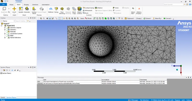
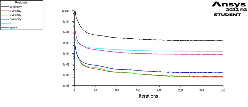
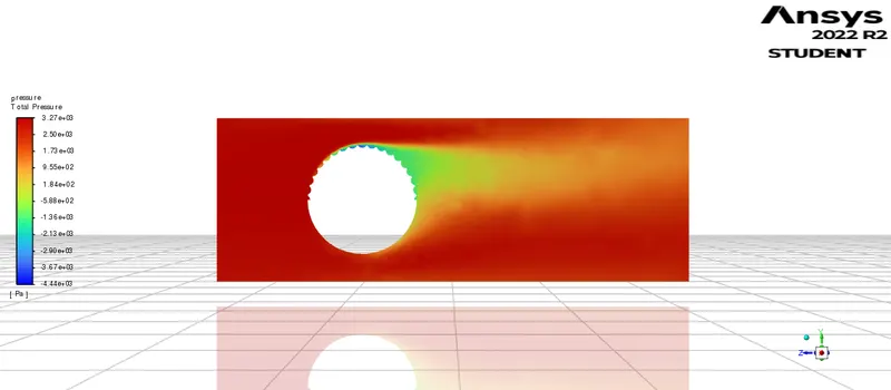
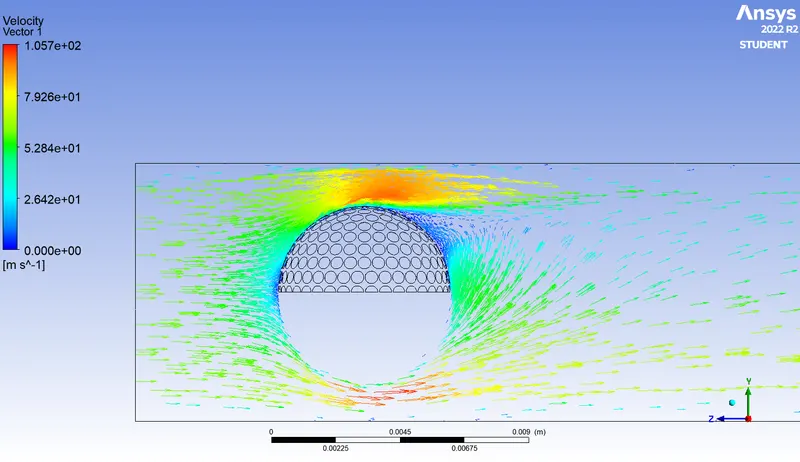
We can identify the direction of the ball by looking at the velocity vectors and claim it's moving down.
The golf ball's dimples serve to minimize drag by minimizing the wake region (recirculation).
It also aids in the attachment of the flow and attempts to detach the flow from the golf ball.
The velocity of the flow beneath the golf ball is high, resulting in low pressure and the formation of a wake following the rough surface. The air velocity on the rough surface is lower, whereas the air velocity on the smooth surface is higher. This causes a pressure differential, which accounts for the ball's downward swing