Week 5 - Turbulence modelling challenge
literature review on Flow analysis around a golf ball
Question: Why the surface of a golf ball is not smooth but rather there are a lot of dents?
Answer: The reason is that those dents called dimples reduce air drag on a golf ball. Such a minuscule difference in the surface helps reduce air drag, and as a result, helps improve the driving distance greatly.
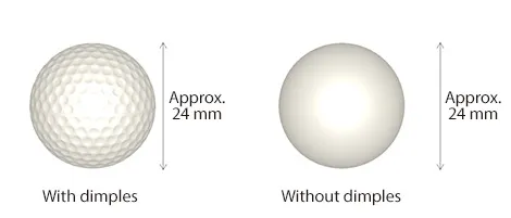
Figure 1: Golf ball with and without dimples
In figure 2, small vortices are generated from the top and bottom of the golf ball. On the other hand, for the case without dimples (figure 3), there is a large vortex behind the golf ball.
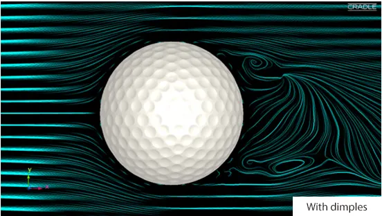
Figure 2: Flow field around golf ball with dimples
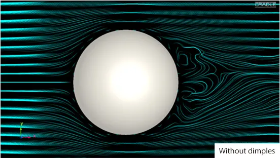
Figure 3: Flow field around golf ball without dimples
Effect of dimples:
Figure 17.1 shows the velocity distribution on a cross-section passing through the middle of the ball. The characteristic of the flow field without dimples is that the flow separates from the ball surface upstream of the ball centerline. That makes the downstream region of flow wider than the ball diameter. This means the air cannot stay along the ball surface because of its momentum.
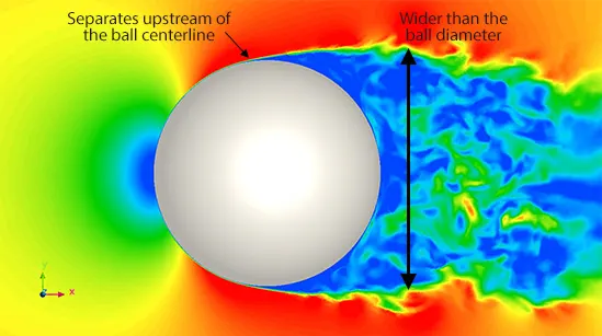
Figure 4: flow field across the golf ball without dimples
Figure 5 shows the velocity distribution with dimples. In the case with dimples, flow along the ball surface keeps staying along the surface past the ball centerline and finally separates downstream. This makes the downstream region of slow flow narrower than the ball diameter.
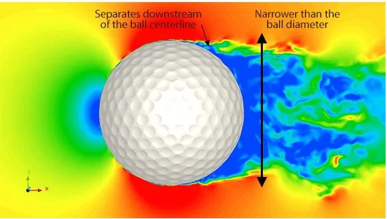
Figure 5: flow field across the golf ball with dimples
Figure 6 shows vortex tubes generated downstream of the ball. Note that only the vortex tubes in the right-hand side of the ball mid-plane are shown. On the left is the case without dimples. We can see that the generation of vortex tubes is initiated somewhat away from the ball surface and that relatively large vortex tubes are generated. On the other hand, in the case with dimples shown on the right, the generation of vortex tubes is initiated on the ball surface. The diameters of the vortex tubes are small compared to those in the case without dimples. We can infer that these many small vortex tubes generated on the ball surface act to mix the air near the ball and the fast-flowing air away from the ball, which in turn shifted the separation point toward downstream. With these differences in the flow fields, the drag coefficient Cd without dimples is 0.53, while Cd with dimples is 0.28. This confirms numerically that the air drag becomes smaller with dimples.
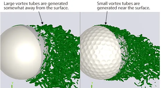
Figure 6: Vortex tube downstream of the ball
Turbulence model:
turbulence modelling is the construction and use of a turbulence model to predict the effect of turbulence. in spite of decades of research, there is no analytical theory to predict the evolution of turbulent flows.
The equations governing turbulent flow can only be solved directly for simple cases of flows. for most real-life turbulent flows, CFD simulations use turbulence models to predict the evolution of turbulence. these turbulence models are simplified constitutive equations, that predict the statistical behaviour of the turbulent flow.
The Navier-Stokes equation governs the velocity and pressure of the fluid flow. in turbulent flow, each of these quantities may be decomposed into the mean part and fluctuating part. Averaging the equations gives the Reynolds-Averaged Navier-Stokes (RANS) equations which govern the mean flow.
However, the nonlinearity of the Navier–Stokes equations means that the velocity fluctuations still appear in the RANS equations, in the nonlinear term  from the convective acceleration. This term is known as the Reynolds stress
What are eddies:
eddy is a swirling of a fluid and reverses current (current in a fluid is a magnitude and direction of flow in that fluid) created when the fluid is in a turbulent regime. The moving fluid creates a space devoid of downstream-flowing fluid on the downstream side of the object. Fluid behind the obstacle flows into the void creating a swirl of fluid on each edge of the obstacle, followed by a short reverse flow of fluid behind the obstacle flowing upstream, toward the back of the obstacle.
Types of eddies: it contains a wide range of turbulent eddy sizes (scale spectrum)
- Large eddies: size/velocity of a large eddy is on the order of mean flow. large eddy derives energy from mean flow. `Size prop L/U`
- smaller eddies: energy is transferred from larger eddies to smaller eddies. in the smallest eddy, turbulent energy is converted into internal energy by viscous dissipation. `SizepropL/(R_e^(3/4)`
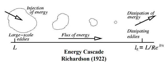
Scales in turbulent flows (Small scale eddies):
- Large eddies transfer energy to the smallest eddies.
- Energy transfer from large eddies must be equal to heat dissipation from small eddies since otherwise, energy at small eddies will be accumulating.
- Assumption that the energy transfer rate is the same at all scales helps establish a scale for small eddies.
- Primary parameters for smallest eddies: mean dissipation (`epsilon`) and kinematic viscosity (`nu`)
- The dimensional argument to establish the following scales of the smallest eddies:
- 1. Length scale (Kolmogorov Scale)
- `etaapprox((nu^3)/epsilon)^(1/4)`
Here, `epsilon=U^3/L`
`etaapprox((nu^3)/(U^3/L))^(1/4)=((mu^3)/(rho^3U^3/L))^(1/4)=((mu^3L^3)/(rho^3U^3/L*L^3))^(1/4)=((L^4)/((rho^3U^3*L^3)/(mu)^3))^(1/4)`
`etaapproxL/(Re)^(3/4)`
Ratio of largest eddy to smallest eddy`=L/eta=Re^(3/4)`
2. Time scale (Kolmogorov Scale)
`t_n=(nu/epsilon)^(1/2)=((mu)/(rhoU^3/L))^(1/2)=(L^2/((rhoUL)/mu))^(1/2)`
`t_n=t/(Re)^(1/2)`
Modelling turbulent flows:
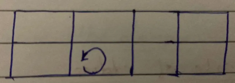
If the size of the vortex is large, this grid can resolve the structure.
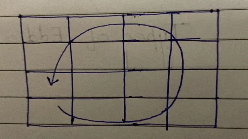
If the size of the vortex is small, then this grid can not be able to resolve the structure. this problem can be solved by reducing the size of the grid. but the problem with this solution is that it is computationally expansive. the basic challenge is to resolve small-scale structures.
Computational approaches to modelling turbulent flow:
- DNS
- LES
- RANS
1. Direct Numerical Simulation (DNS):
- Navier-Stokes equations are numerically solved without any turbulence model.
- For the Reynolds numbers encountered in most industrial applications, the computational resources required by a DNS would exceed the capacity of the most powerful computer currently available. However, direct numerical simulation is a useful tool in fundamental research in turbulence.
- Using DNS it is possible to perform "numerical experiments", and extract from them information difficult or impossible to obtain in the laboratory, allowing a better understanding of the physics of turbulence.
- DNS are useful in the development of turbulence models for practical applications, such as sub-grid scale models for LES and models for methods that solve the RANS. This is done by means of "a priori" tests, in which the input data for the model is taken from a DNS simulation, or by "a posteriori" tests, in which the results produced by the model are compared with those obtained by DNS.
- Computational cost is very high even at a low Reynolds number. Not practical for industrial flows.
- DNS is not available in FLUENT.
2. Large Eddy Simulation (LES):
- Large eddies are directly resolved but eddies smaller than mesh are modelled.
- Less expansive than DNS but the amount of computational resources and efforts are still too large for most practical applications.
3. Reynolds Averaged Navier-Stokes Equations (RANS):
- RANS equations are the time-averaged equations of motion for fluid flow. the idea behind the equations is Reynolds decomposition, whereby the instantaneous quantity is decomposed into its time average and fluctuating quantities.
- `rhobaru_j((delbaru_i)/(delx_j))=rhobarf_i+del/(delx_j)[-barpdelta_(ij)+mu((delbaru_i)/(delx_j)+(delbaru_j)/(delx_i))-rhobar(u_i^'u_j^')]`
Derivation of RANS equations:
- The basic tool required to derive the RANS equations from the instantaneous Navier-Stokes equation is the Reynolds decomposition.
`ubrace(u(x,t))=ubrace(baru(x))+ubrace(u^'(x,t))`
Instantaneous component=Time-average component + Fluctuating component
where, x=(x,y,z)=position vector
For incompressible Newtonian fluid,
Continuity equation:
`(delu_1)/(delx_1)+(delu_2)/(delx_2)+(delu_3)/(delx_3)=0`
From Reynolds decomposition, `u=baru+u^'`
`(del(baru_1+u_1^'))/(delx_1)+(del(baru_2+u_2^'))/(delx_2)+(del(baru_3+u_3^'))/(delx_3)=0`
By using Reynolds Operator, `((delphi)/(delx))=(del(phi))/(delx) & ((delphi)/(delt))=(del(phi))/(delt)`
`(delbaru_1)/(delx_1)+(delu^')/(delx_1)+(delbaru_2)/(delx_2)+(delu^')/(delx_2)+(delbaru_3)/(delx_3)+(delu^')/(delx_3)=0`
Time-averaging this equation yields,
`bar(delbaru_1)/(delx_1)+bar(delu^')/(delx_1)+bar(delbaru_2)/(delx_2)+bar(delu^')/(delx_2)+bar(delbaru_3)/(delx_3)+bar(delu^')/(delx_3)=0` ----------(1)
We know that, `barphi=1/Tlim_(t->oo)int_t^(t+T)phidT`
Consider `phi=(delbaru_1)/(delx_1)`
`bar(delbaru_1)/(delx_1)=1/Tlim_(t->oo)int_t^(t+T)(delbaru_1)/(delx_1)dT`
`bar(delbaru_1)/(delx_1)=1/Tlim_(t->oo)del/(delx_1)int_t^(t+T)baru_1dT`
`bar(delbaru_1)/(delx_1)=del/(delx_1)1/Tlim_(t->oo)int_t^(t+T)baru_1dT`
`bar(delbaru_1)/(delx_1)=del/(delx_1)barbaru_1`
From equation (1),
`(delbarbaru_1)/(delx_1)+(delbar(u^'))/(delx_1)+(delbarbaru_2)/(delx_2)+(delbar(u^'))/(delx_2)+(delbarbaru_3)/(delx_3)+(delbar(u^'))/(delx_3)=0` ----------(2)
Properties: 1. Time average of an average quantity is same (`barbar(u)=baru`). 2. Mean of the fluctuating quantity is equal to zero (`bar(u^')=0`) hence equation 2 becomes
`(delbaru_1)/(delx_1)+(delbaru_2)/(delx_2)+(delbaru_3)/(delx_3)=0`
X-Momentum equation:
`(delu_i)/(delt)+u_j(delu_i)/(delx_j)=-1/rho(delp)/(delx_i)+nu(del^2u_i)/(delx_jdelx_j)`(N-S Equation)
By applying Reynolds decomposition, the momentum equation yields
`(delbaru_i)/(delt)+baru_j(delbaru_i)/(delx_j)=-1/rho(delbarp)/(delx_i)+nu(del^2baru_i)/(delx_jdelx_j)-(delbar(u_i^'u_j^'))/(delx_j)`
On further manipulation this yields
`rho(delbaru_i)/(delt)+rhobaru_j(delbaru_i)/(delx_j)=del/(delx_j)[-barpdelta_(ij)+2mubardelta_(ij)-rhobar(u_i^'u_j^')]`----------(3) (RANS Equation)
Here,
`bardelta_(ij)=1/2[(delbaru_i)/(delx_j)+(delbaru_j)/(delx_i)]` is the mean rate of strain tensor.
`-rhobar(u_i^'u_j^')=R_(ij)` = Reynold Stress Term
Note: From equation (3), it shows that velocity fluctuations still appear in the RANS equations, in the nonlinear term `-rhobar(u_i^'u_j^')`
This nonlinear Reynold stress term requires additional modelling to close the RANS equation for solving and has lead to the creation of different turbulence models
Closure Problem:
To obtain equations containing only the mean velocity and pressure, we need to close the RANS equations by modelling the Reynolds stress term `R_(ij)` as a function of the mean flow, removing any reference to the fluctuating part of the velocity. This is the closure problem.
Eddy Viscosity:
Joseph Valentin Boussinesq was the first to attack the closure problem by introducing the concept of eddy viscosity.
`-bar(u_i^'u_j^')=nu_t[(delbaru_i)/(delx_j)+(delbaru_i)/(delx_j)]-2/3kdelta_(ij)` ( Boussinesq hypothesis)
`-bar(u_i^'u_j^')=2nu_tS_(ij)-2/3kdelta_(ij)`
Here,
`nu_t` = Turbulence eddy viscosity
`S_(ij)` = Mean rate of strain tensor
`k=1/2bar(u_i^'u_i^')` = Turbulence kinetic energy
`delta_(ij)` = Kronecker delta
Prandtl's mixing length concept:
Later Ludwig Prandtl introduced the concept of mixing length, along with the idea of the boundary layer. for wall-bounded turbulent flow eddy viscosity must vary with distance from the wall.
`nu_t=|(delu)/(dely)| l_m^2`
Calculation of Turbulence viscosity (`nu_t`):
The Boussinesq hypothesis is employed in the Spalart-Allmaras (S-A), k-epsilon (`k-epsilon`)and k-omega (`k-omega`)models and offers a relatively low computational cost for turbulence viscosity (`nu_t`)
| Turbulence Model Available in FLUENT(To model the Reynold stress term) | |||
| First-order model | Second-order model | ||
| 1. | Zero equation model (Mixing length) | 1. | Algebraic stress model |
| 2. | One equation model (Spalart Allmaras) | 2. | Reynold stress model |
| 3. | Two equation model(k-Omega & k-epsilon) | ||
First-order model: Uses first-order partial differential equation (PDE) to solve kinematic turbulence viscosity (`nu_t`).
1. Zero equation model:
- Mixing length model
- No PDE is used to solve `nu_t`
- Directly solve `nu_t`using mixing length model
2. One equation model:PDE is used for solving turbulent kinetic energy to obtain `nu_t`
-
Spalart-Allmaras turbulence model:
- The Spalart–Allmaras model was developed for aerodynamic flows. It is not calibrated for general industrial flows.
3. Two equation model:
- Most commonly used method in industries
- Two PDEs are used to solve for:
- Turbulent kinetic energy (`k`) and dissipation rate of turbulent kinetic energy (`epsilon`)
- Turbulent kinetic energy (`k`) and specific dissipation rate (`omega`)(of the turbulence kinetic energy k into internal thermal energy).
`k-epsilon` turbulence model:
- the k-ε model focuses on the mechanisms that affect the turbulent kinetic energy.
- Standard `k-epsilon` turbulence model:
- The exact k-ε equations contain many unknown and unmeasurable terms. For a much more practical approach, the standard k-ε turbulence model (Launder and Spalding, 1974) is used.
- Realizable `k-epsilon` turbulence model:
- Renormalized group (RNG) `k-epsilon` turbulence model:
`k-omega` turbulence model:
- Standard `k-omega` turbulence model
- SST `k-omega` turbulence model
Simulation:
The analysis is performed with a model shown in Figure 2, where a golf ball is placed inside a rectangular box of air. Although golf balls fly through the air, in reality, the ball is fixed in space and the air is blown in at the flying speed of the golf ball. In this analysis, the flying speed of 60 m/s is assumed.
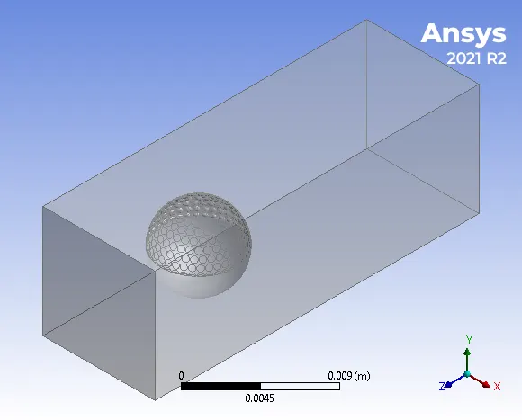
Figure 7: Geometry open in Design Modeler
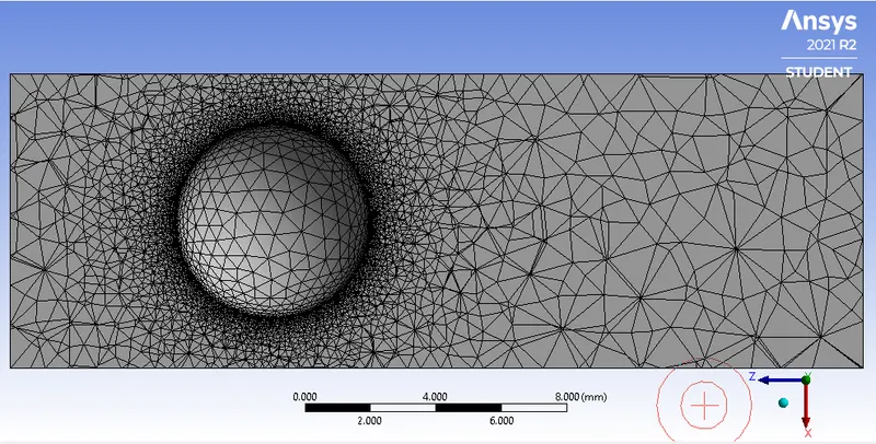
Figure: Default Meshing
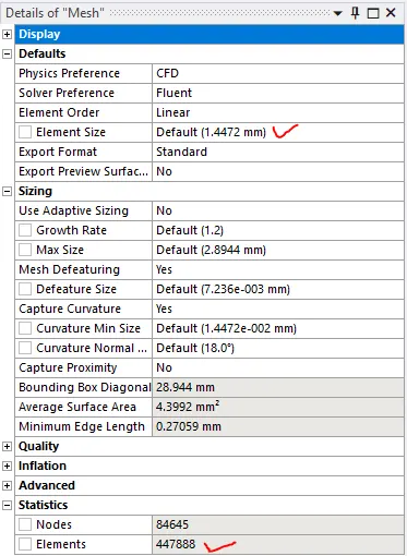
Figure: Mesh details
Named Selection: To provide the boundary conditions, we give the name selection like inlet, outlet, symmetry surfaces, and golf ball.
Estimating Reynolds Number
`R_e=(rho UL)/mu`
Where:
`rho`= Fluid density
U= Characteristic velocity
L= Characteristic length=Gulf ball diameter D
`mu`= Dynamic viscosity of the fluid
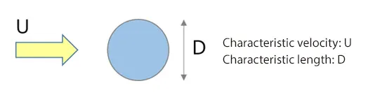
Figure: Characteristic velocity and Characteristic length for a flow around the ball
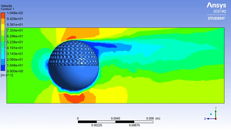
Figure: Velocity contour plot
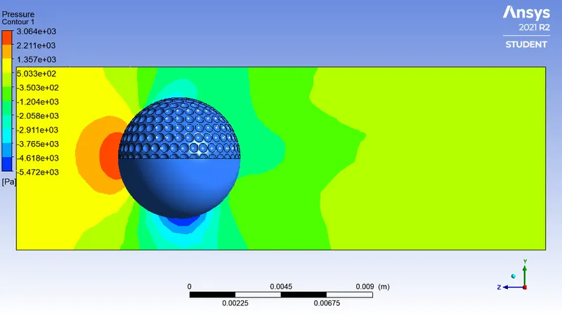
Figure: Pressure contour plot
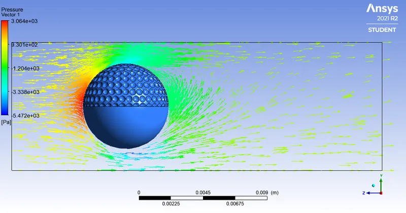
Figure: Pressure vector plot
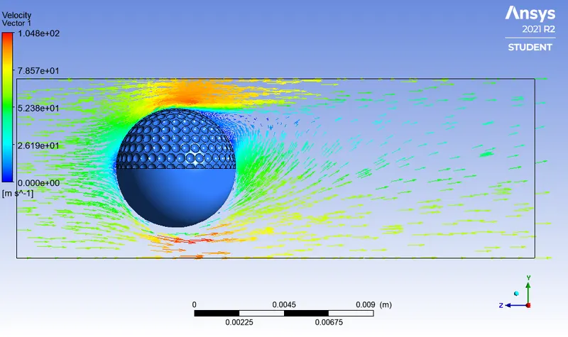
Figure: Velocity vector plot