Simulation of Rayleigh Taylor Instability

AIM:

The aim of this project is to simulate Rayleigh-Taylor instability using ANSYS FLUENT.

OBJECTIVES OF THE PROJECT:

• Perform the Rayleigh Taylor instability simulation for 2 different mesh sizes with the base mesh being 0.5 mm.
• Create animations of the results and compare the results by showing the animations.
• Find out the effect of mesh size on simulation.
• Run another simulation with water and user-defined material(density = 400 kg/m³, viscosity = 0.001 kg/m-s) for refined mesh.
• Define the Atwood Number. Find out the Atwood number for both the cases and explain how the variation in Atwood number in the above two cases affects the behavior of the instability.

THEORY:

Taylor instability

The Rayleigh-Taylor instability, or RT instability, is an instability of an interface between two fluids of different densities which occurs when the lighter fluid is pushing the heavier fluid. Examples.

• Behavior of water suspended above oil in the gravity of earth.
• Mushroom clouds like those from volcanic eruptions and atmospheric nuclear explosions.

Some practical CFD models based on mathematical analysis of Rayleigh waves

• Turbulent mixing modelling by Rayleigh-Taylor instability

Rayleigh-Taylor instability occurs when a perturbed interface between two fluids of different density is subjected to a normal pressure gradient,Taylor.If the pressure is higher in the light fluid than in the dense fluid the differential acceleration produced causes the two fluids to mix.

Direct two-dimensional numerical simulation and experiments, in which small rocket motors accelerate a tank containing two fluids, have been used to investigate turbulent mixing by Rayleigh-Taylor instability at a wide range of density ratios. The experimental data obtained so far has been used to calibrate an empirical model of the mixing process which is needed to make predictions for complex applications. The model devised, which is a form of turbulence model, is based on the equations of multiphase flow. These equations describe velocity separation arising from the action of a pressure gradient on fluid fragments of different density. The dissipation arising from the drag between the fluid fragments is treated as a source of turbulence kinetic energy which is then used to define turbulent diffusion coefficients. Gradient diffusion processes are thereby included in the model.

• Non-ideal Rayleigh Tayor mixing

Rayleigh-Taylor mixing is a classical hydrodynamic instability that occurs when a light fluid pushes against a heavy fluid. The two main sources of nonideal behavior in Rayleigh-Taylor (RT) mixing are regularizations (physical and numerical), which produce deviations from a pure Euler equation, scale invariant formulation, and nonideal (i.e., experimental) initial conditions. The Kolmogorov theory of turbulence predicts stirring at all length scales for the Euler fluid equations without regularization. We interpret mathematical theories of existence and nonuniqueness in this context, and we provide numerical evidence for dependence of the RT mixing rate on nonideal regularizations; in other words, indeterminacy when modeled by Euler equations. Operationally, indeterminacy shows up as nonunique solutions for RT mixing, parametrized by Schmidt and Prandtl numbers, in the large Reynolds number (Euler equation) limit. Verification and validation evidence is presented for the large eddy simulation algorithm used here. Mesh convergence depends on breaking the nonuniqueness with explicit use of the laminar Schmidt and Prandtl numbers and their turbulent counterparts, defined in terms of subgrid scale models. The dependence of the mixing rate on the Schmidt and Prandtl numbers and other physical parameters will be illustrated. We demonstrat numerically the influence of initial conditions on the mixing rate. Both the dominant short wavelength initial conditions and long wavelength perturbations are observed to play a role. By examination of two classes of experiments, we observe the absence of a single universal explanation, with long and short wavelength initial conditions, and the various physical and numerical regularizations contributing in different proportions in these two different contexts.

PROCEDURE:

Creating the geometry

We first create the geometry in spaceclaim. To create the rayleigh taylor instability flow. we create two boxes of same dimension one on top of another as follows.

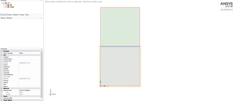
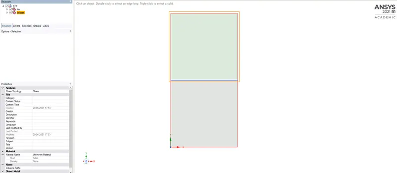
We start with creating 2 boxes as shown and use the share option under workbench tab this will make sure that the topologies are shared.

Once the geometry is created we close spaceclaim, The geometry will be updated on to workbench.

Meshing

In the mesher, we first create a base line mesh by simply clicking the mesh button. But usually this will be a coarse mesh hence we use a mesh size of 0.5mm

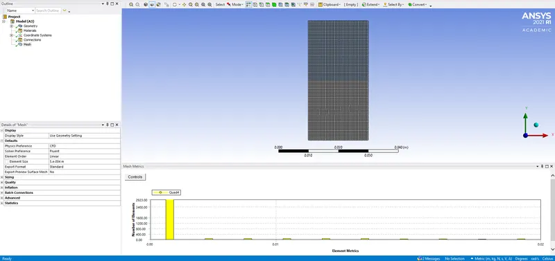
We now press the update button which will export this mesh into the fluent workbench.

Case Setup

In the solver, we choose a transient state, pressure based solver. we will not be solving for energy in this case.

Since gravity is involved in the phenomena we input the gravity according to the geometry orientation i.e., in the -ve y direction as 9.81 m/s^2

The type of turbulence model used here is laminar.

Materials are

Fluid - air

Fluid - water

Since this flow involves two types of fluids with different phases we enable the multiphase option. In the multiphase tab we select the volume of fluid method.

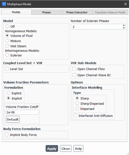
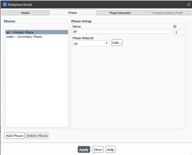
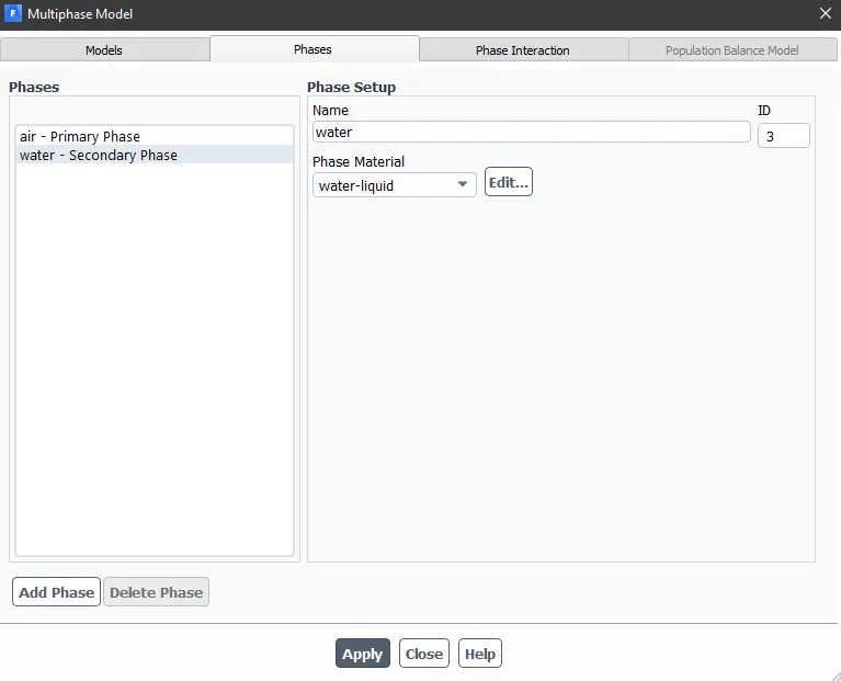
before we proceed further it is to be remembered that during the meshing of the geometry we didnt specify any names/BC's. So we need to be careful while assigning the inputs to the regions.

Now we initialise the solution using the standard initialisation method and set some monitors to capture the contour of volume fraction of water. We also save this animation as we capture it.

Before proceed into calculation we need to patch the regions. i.e., we specify the volume fraction in the regions

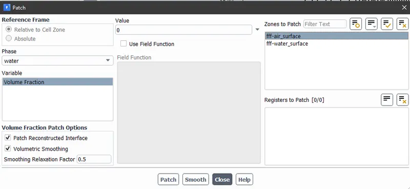
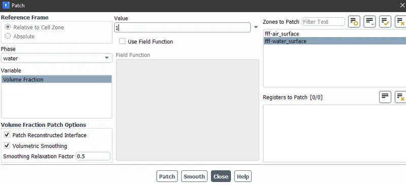
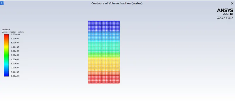
We can verify that the correct values are assigned by checking the volume fraction of water on the geometry

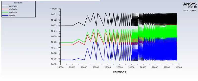
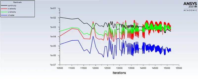
After everything is set we run the simulation for 1500 no of time steps with a time step size of 0.005s. Once the solution has converged we get the following results.

Residual plot

Volume fraction of water

Video animation

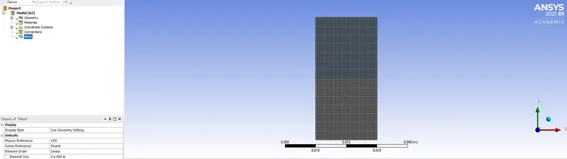
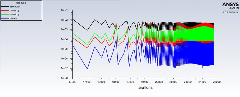
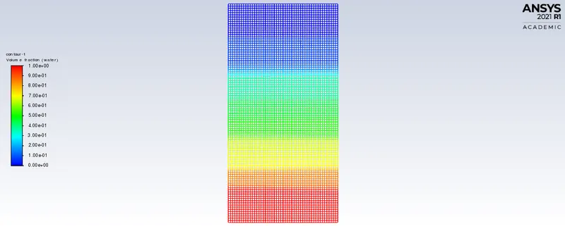
To see the effect of grid size on the solution we create another case with the same setup but a change of mesh to 0.4 mm

For a grid size of 0.4mm

Mesh

Residual plot

Volume fraction Contour

Video animation

Now we change the material properties such as density, viscosity to see if a change in material will change the end result or not.

For a change in material property

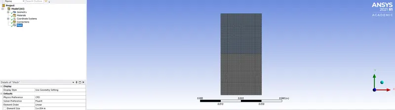
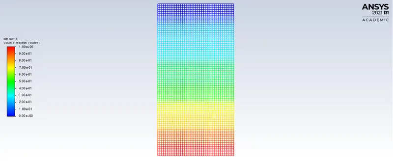
With the same setup as above baseline setup we changed the material properties, density to 400kg/m^3 and viscosity to 0.001 kg/m-s

mesh size

Residual plot

volume fraction contour

video animation

Atwood Number

The Atwood number (A) is a dimensionless-number in fluid dynamic, used in the study of hydrodynamic instabilites in density stratified flows. It is a dimensionless density ratio defined as

`A = {rho_1 - rho_2}/{rho_1+rho_2}`

where

`rho_1 is the density of heavier fluid

`rho_2`is the density of lighter fluid

• For Atwood number closer to 0,means Rayleigh Taylor instability fluid flow take the form asymmetric finger of fluid.
• For Atwood number closer to 1,means the lighter fluid below the heavier fluid take the form of larger bubble-likes plumes

Atwood number for standard air and water

`rho_1 = 1000`

`rho_2 = 1.225`

`A = {1000 - 1.225)/(1000 + 1.225)`

A = 0.997

Atwood number for standard air and water

`rho_1 = 400`

`rho_2 = 1.225`

`A = {400 - 1.225)/(400 + 1.225)`

A = 0.993

CONCLUSION

The following conclusions have been made after observing the above plots and results

• The size of the bubble and time taken to settle down seem to be constant even with the mesh but the interface is much sharp with the fine mesh.
• However, the with the second fluid the size of the bubble and time taken seem to be reduced. From the definition of atwood number we can see that as the number moves far from 1 towards 0 the instability of the fluid decreases.
• The reason we didnt choose the steady state solver is because we are interested not only on the end solution but also the path taken to the end solution. Hence for our application steady state solver is not recommended.

REFERENCES

• https://en.wikipedia.org/wiki/Rayleigh%E2%80%93Taylor_instability
• https://en.wikipedia.org/wiki/Atwood_number