Week 5 - Rayleigh Taylor Instability
Objective :
1) Name few practical CFD models based on analysis of Rayleigh Taylor waves . Explain how they have been adapted for CFD calculations.
2) Perform Rayleigh Taylor simulations for 2 mesh sizes with base mesh .5mm . Upload animations for the same and explain the effect of mesh size on the simuation . Explain why steady state simulations are not suitable for this type of simulations.
3) Run one more simulation with a user defined material and water .
4) Define the Atwood Number. Find out the Atwood number for both the cases and explain how the variation in Atwood number in the above two cases affects the behavior of the instability.
Theory:
The Rayleigh-Taylor instability is an instability of the interface separating two immiscible fluids ; the densest of which rests on the lightest. Following a disturbance of the interface, the dense fluid enters the light fluid.
The interface growths with a characteristic “mushroom” shape. For example, Rayleigh-Taylor instability manifests itself in several areas such as astrophysics with the Crab Nebula, thermonuclear fusion with laser implosion of deuterium-tritium targets, or meteorology with cloud formation.
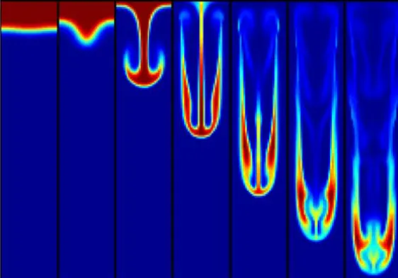
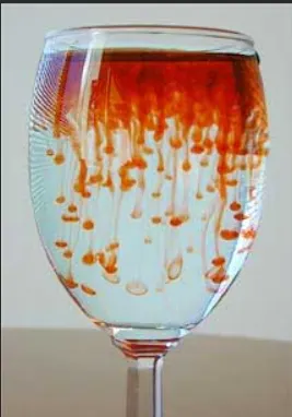
Therea are several types of models based on Rayleigh Taylor instabilities. A few of them are described below.
1) Richtmyer–Meshkov instability (RMI)
The Richtmyer–Meshkov instability (RMI) occurs when two fluids of different density are impulsively accelerated. Normally this is by the passage of a shock wave. The development of the instability begins with small amplitude perturbations which initially grow linearly with time. This is followed by a nonlinear regime with bubbles appearing in the case of a light fluid penetrating a heavy fluid, and with spikes appearing in the case of a heavy fluid penetrating a light fluid. A chaotic regime eventually is reached and the two fluids mix. This instability can be considered the impulsive-acceleration limit of the Rayleigh-Taylor instability.
2) Kelvin–Helmholtz instability
The Kelvin–Helmholtz instability typically occurs when there is velocity shear in a single continuous fluid, or additionally where there is a velocity difference across the interface between two fluids. A common example is seen when wind blows across a water surface; the instability constant manifests as waves. Kelvin-Helmholtz instabilities are also visible in the atmospheres of planets and moons, such as in cloud formations on Earth or the Ref Spot on Jupiter, and the atmospheres coronas of stars, including the Sun's.
3) Plateau–Rayleigh instability
The Plateau–Rayleigh instability, often just called the Rayleigh instability, explains why and how a falling stream of fluid breaks up into smaller packets with the same volume but less surface area. It is related to the Rayleigh-Taylor Instability and is part of a greater branch of fluid dynamics concerned with fluid thread break up. This fluid instability is exploited in the design of a particular type of ink jet technology whereby a jet of liquid is perturbed into a steady stream of droplets .The driving force of the Plateau–Rayleigh instability is that liquids, by virtue of their surface tensions, tend to minimize their surface area. A considerable amount of work has been done recently on the final pinching profile by attacking it with self-similar solutions.
Set up :
1) Geometry
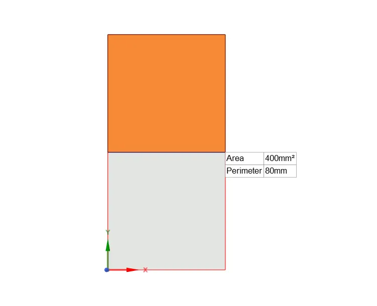
Two squares of 20x20mm dimesions were created along the xy plane in 2 components . Pull tool was used extract surfaces . Topology was set to shared .
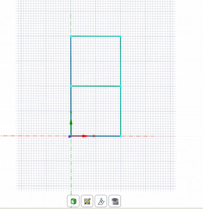
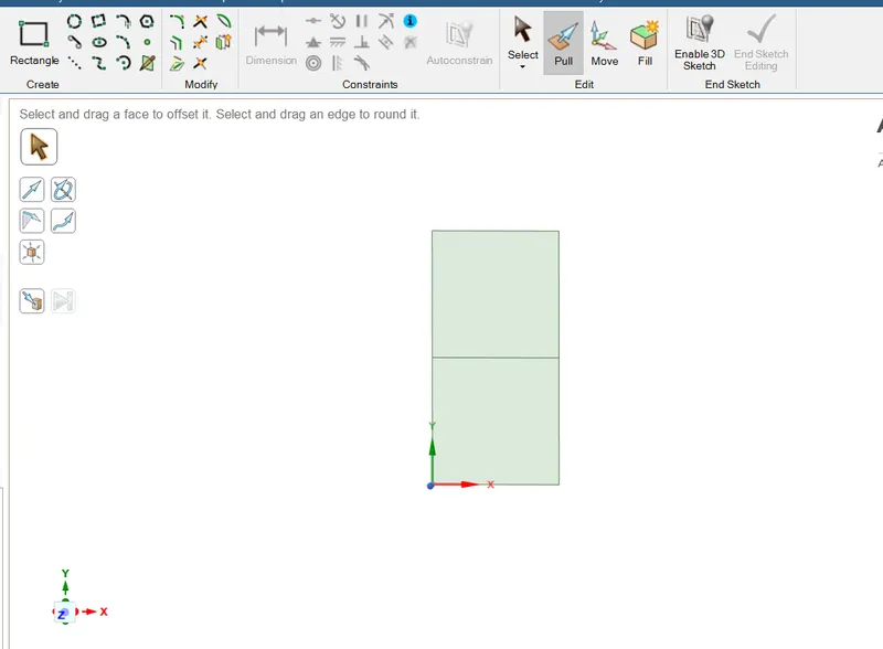
Share tool from workbench was used to share common edge.
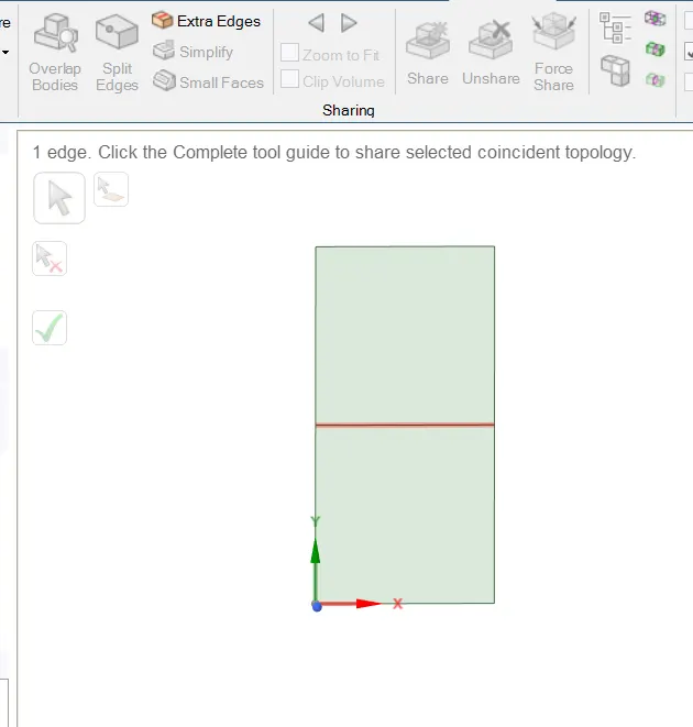
Thus the final geometry was obtained .
2)Meshing
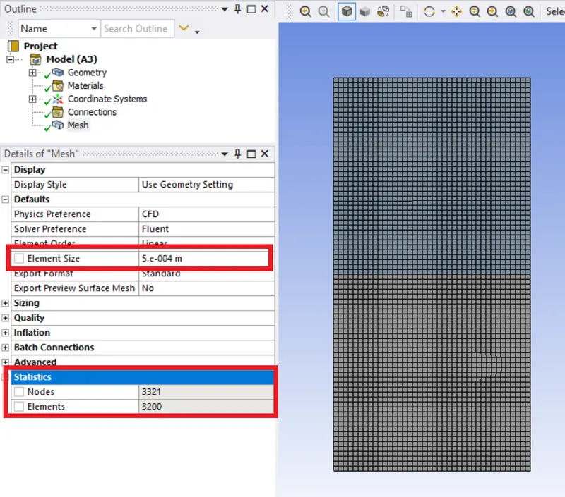
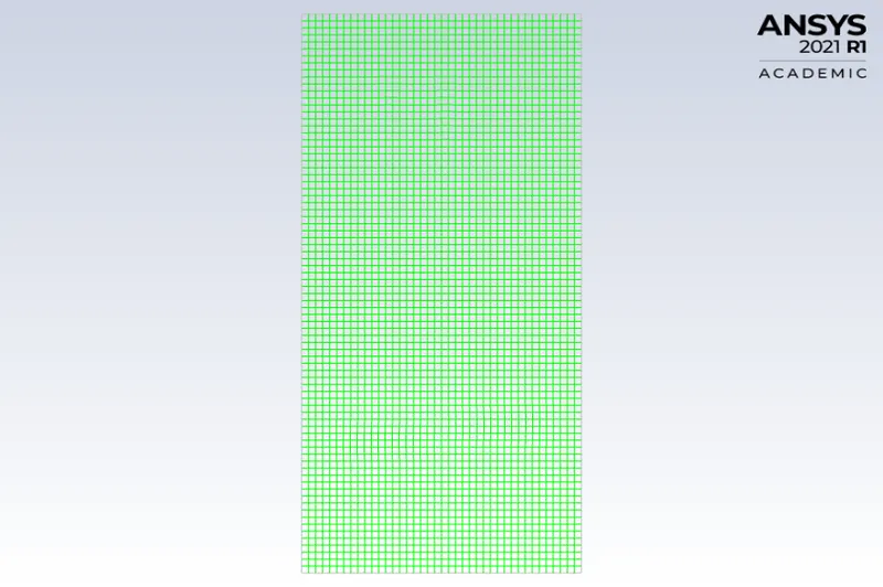
Meshing module was opened and element size was set to .5mm for 1st case , .25mm for 2nd and 3rd case respectively .
3)Set up
The mesh was updated and set up module was opened with double precision and 4 core usage.
The general time setting was changed to transient and gravity was introduced along y axiz.
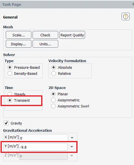
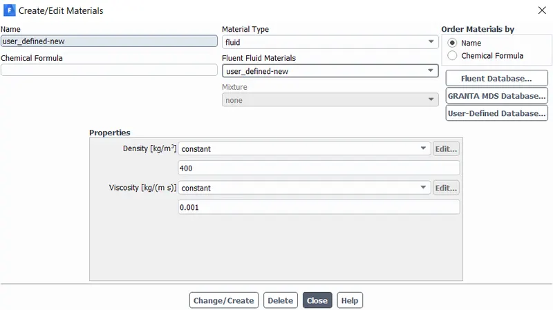
Material was selected as air and water for case 1 and 2 . For case 3, a user defined material was introduced with density 400kg/m^3 and viscosity .001 kg/m-s .
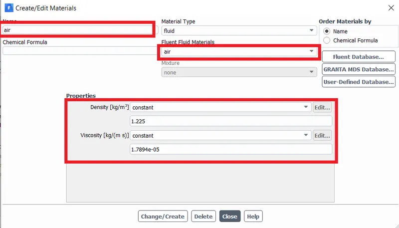
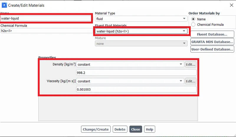
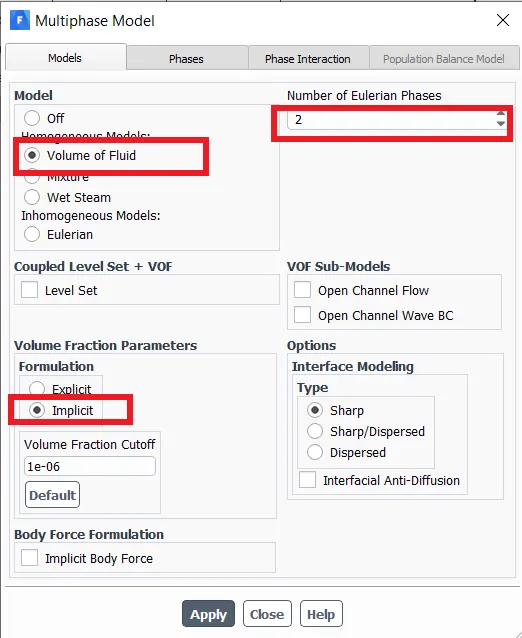
Turbulence model was set to multiphase and energy equation was not turned on . Within this , the phases were also defined.
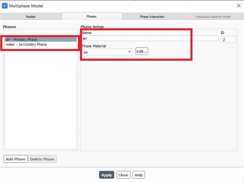
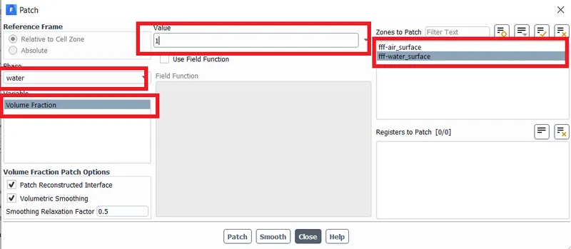
The solution was initialized in standard model . The volumes were patched respectively.
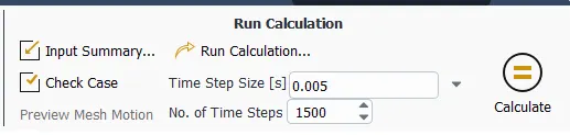
The solution was run for 1500 timesteps with .005 timestep size .
Results :
Case 1:
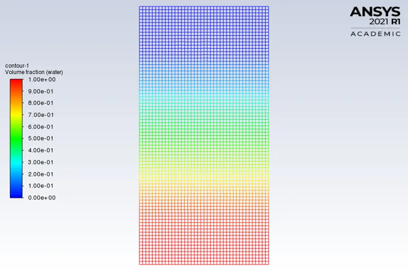
Mesh size : 0.5mm
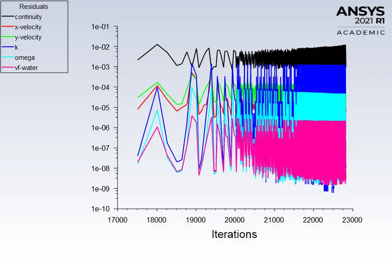
Scaled Residuals
Contour for steady state volume fraction.
link :https://drive.google.com/file/d/1yN3IBgjrW9tkeDf-ZmN0akNiM1Ql2q9o/view?usp=sharing
Case 2:
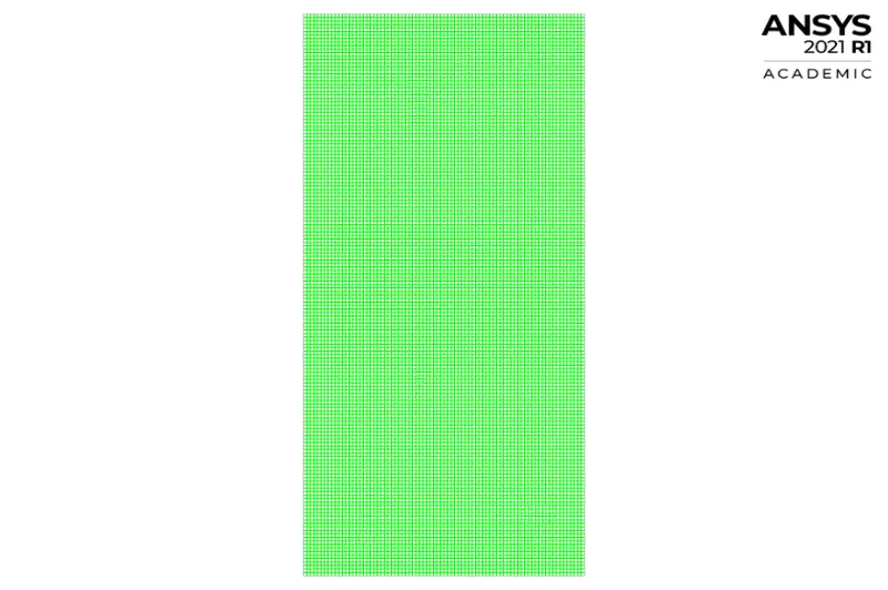
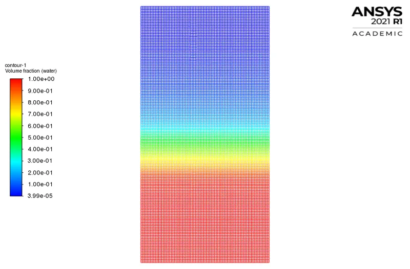
Mesh size : .25mm
Mesh
Contour for steady state volume fraction
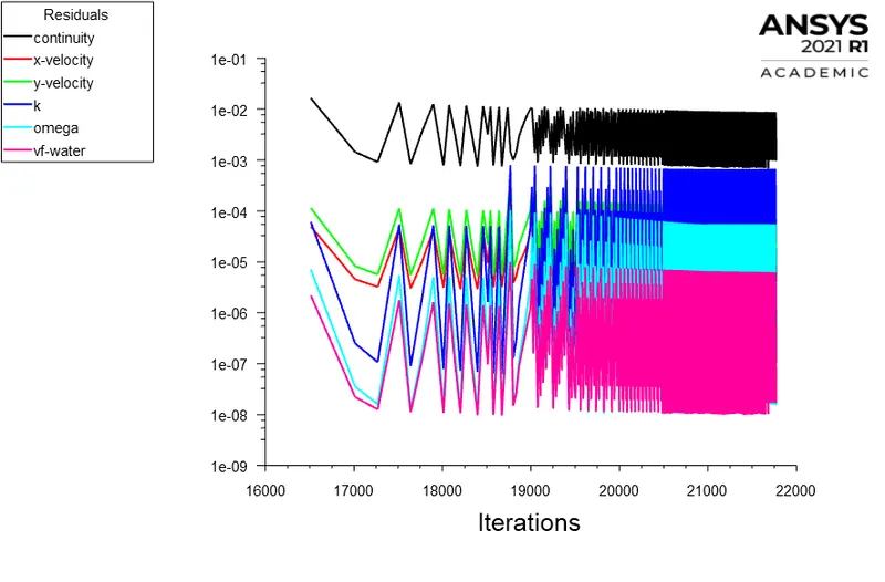
Scaled residuals
limk:https://drive.google.com/file/d/1bE1vv8IPMNHuifWErmadAJ3LVeBejp1s/view?usp=sharing
Case 3
mesh size: .25 mm
material:
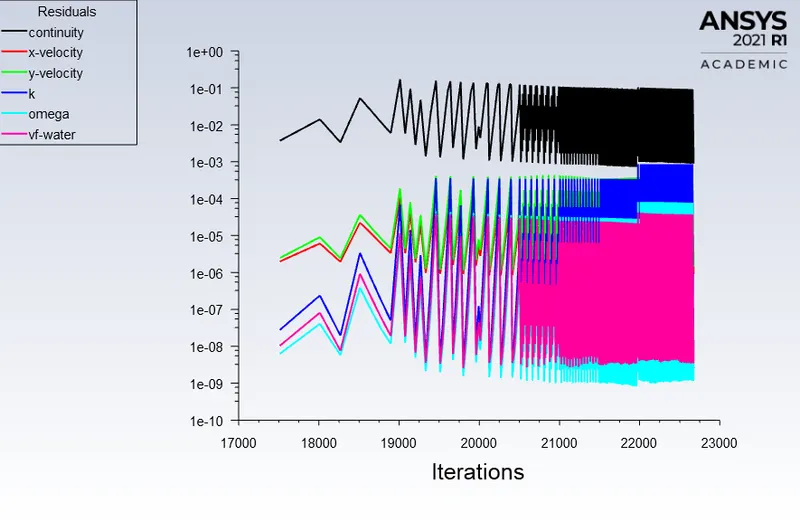
Scaled residuals
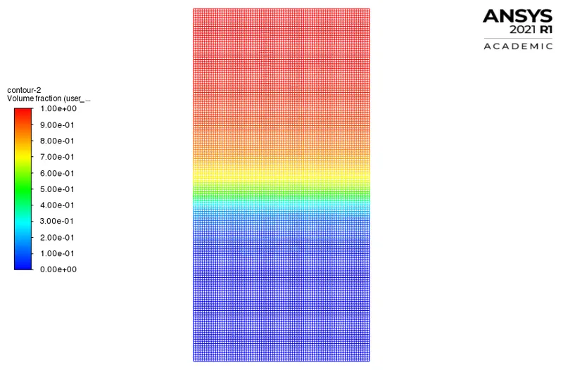
Contour for steady state volume fraction
link:https://drive.google.com/file/d/1TO1Exb5vXOhpxA-bKy5aYTeLaNgScd43/view?usp=sharing
Conclusion:
1) We can observe that , as the mesh refinement increases, the time taken to take reach state increases .The instabilities formed are much more smaller in case of refined mesh . Hence the interface breaks down takes longer for a refined mesh .
2)
The Atwood number (A) is a dimensionless number in fluid dynamics used in the study of hydrodynamic instabilities in density stratified flows. It is a dimensionless density ratio defined as
`A= (rho_1-rho2)/(rho_1+rho_2)`
- where
- `rho_1 =` Density of heavier fluid
- `rho_2`= Density of lighter fluid
In case 1&2
`rho_1=1000`
`rho_2= 1.225`
A= 1000-1.225/1000+1.225 = 0.9975
In case 3
`rho_1=1000`
`rho_2= 400`
A= 1000-400/1000+400= 0.4285
We can observe that as the Atwood number decreases, the time taken to reach steady state also decreases. In case 3, the user defined fluid was much denser(or more viscous ) hence the formation of instabilities were quite low and reached a steady state quite fas compared to other 2 cases since the difference between density of the 2 fluids are less.
3) We cannot use steady state approach for these types of simulations as we need to study the change with respect to time , which is possible only in transient simulations.