Week 5 - Rayleigh Taylor Instability
Instability:
Instability is something where and when it starts to grow, and it eventually continues to grow and they are triggered by accidental disturbances between the mediums. One such instability we will analyze in this challenge is Rayleigh-Taylor Instability.
What is Rayleigh-Taylor Instability?
Rayleigh-Taylor Instability occurs when there are at least 2 different mediums with differing densities where the higher-density fluid stays at the top and the lower-density fluid stays below it. When they are stable, and if we cause any perturbations or disturbances, then the fluid with high density which has higher potential energy forms a spike shape coming down, thus converting into kinetic energy, towards the bottom, and the low-density fluid forms a bubble and moves upwards. This type of Instability caused between 2 different mediums is termed as Rayleigh-Taylor Instability.
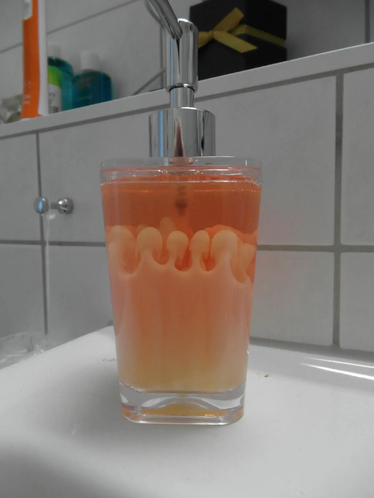
Some practical CFD models based on the mathematical analysis of Rayleigh Taylor waves are 1. Kelvin-Helmholtz Instability, 2. Plateau-Rayleigh Instability and 3. Richtmyer-Meshkov Instability. Let us see about those in detail.
1. Kelvin-Helmholtz Instability:
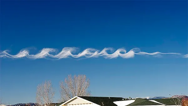
When a relative motion is present between different mediums, there will be a velocity shear, forming a small wave-like pattern. And due to Bernoulli's principle, the waves deform based on the pressure difference and thus cause a wholesome instability. This will clearly be evident in clouds.
2. Plateau-Rayleigh Instability:
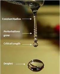
The best example of this instability is the jet stream of water breaking apart as liquid droplets as soon as it leaves the outlet. The jet stream always tends to be in a lower state of energy. The energy state is in accordance with the surface area. The small droplets have less surface area and hence the jet tends to take its shape. This type of instability is called Rayleigh Taylor Instability.
3. Richtmyer-Meshkov Instability:
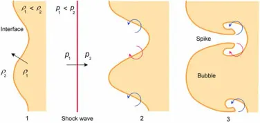
When a shock wave interacts with the interface between different mediums, then instability occurs, and such a kind of instability is called Rayleigh Taylor instability.
Rayleigh Taylor Instability Case setup:
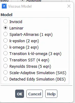
Here the flow is considered to be laminar since it only involves 2 fluids air and water.
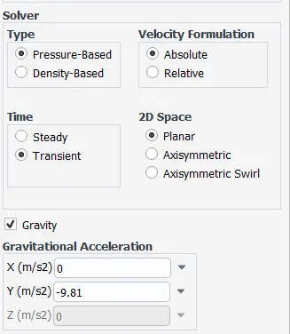
The solver used is a Pressure based one, and we use a transient(time-dependent) solver for this setup instead of a steady-state solver. The reason is that, if we are in need of the final result, the steady state solver would be good to go type, but our area of interest is capturing the dynamic behavior of the fluids under gravity which varies with respect to time.
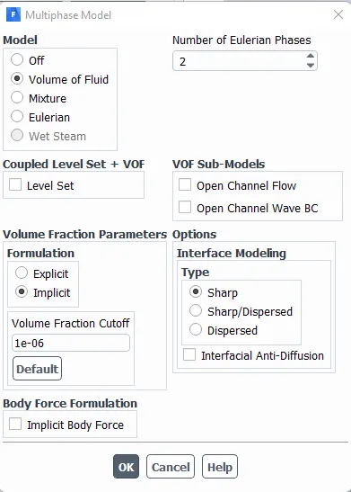
Then we select the multiphase model since it involves different mediums, and select the implicit equation. The reason for selecting the implicit equation is that it does not contain the artificial diffusivity term(Courant number) forming the CFL(Courant–Friedrichs–Lewy) condition, whereas the explicit equation contains it so which there is a high possibility to get a diverged result due to improper inputs like grid spacing or time step size.
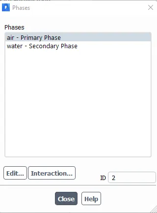
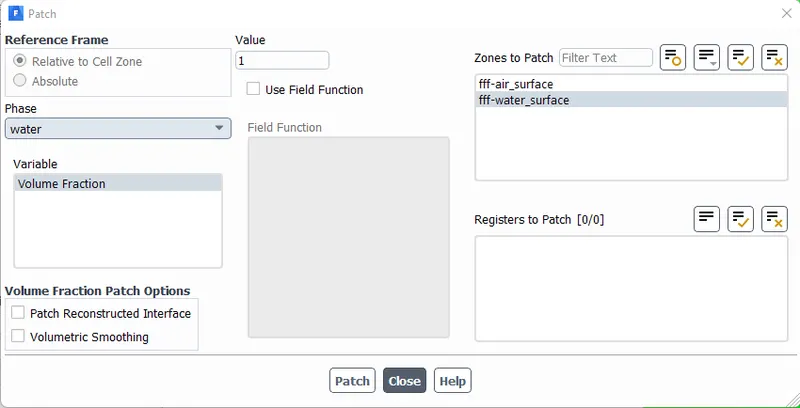
We should impart the primary and secondary phases. In this case, it is air and water respectively. That is, here if we generalize air as the primary phase, then at the next stage of setup, when we use "PATCH" option, we will be having an option to choose the volume fraction of water in the desired region.
And then we must patch the water-based region with the volume fraction of water with the value of 1, and for air with the value of 0, in order to give the air and water phase regions their complete volume fraction.
Result:
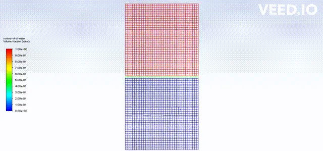
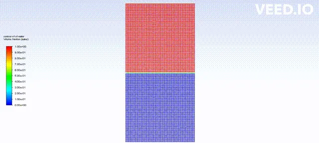
The contour under the phases for the volume fraction is created and animation is set up. And the time-step size is given as 0.005 and the total time steps were inputted as 500s.
Animation:
0.5mm:
0.25mm:
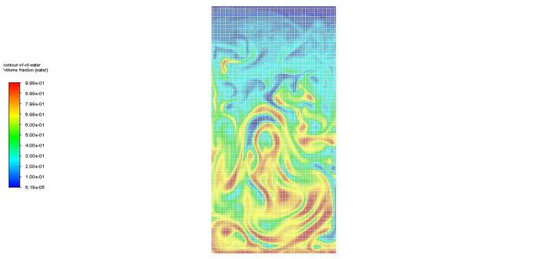
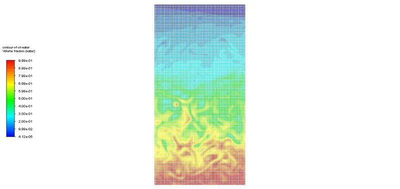
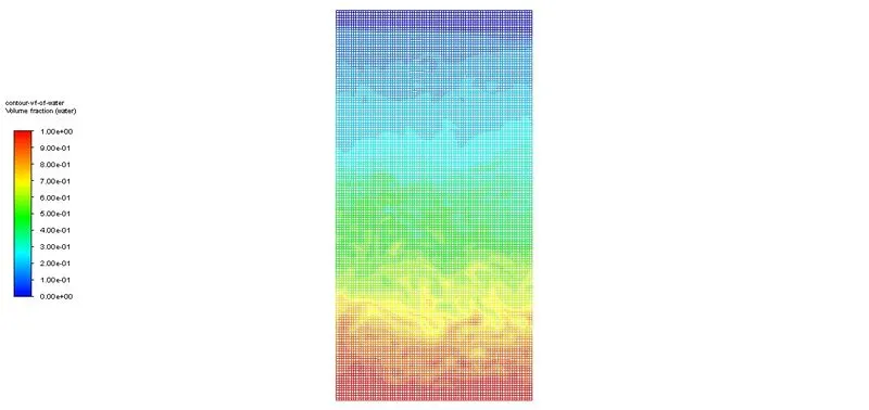
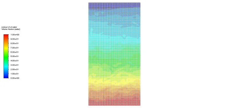
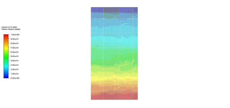
The effect of Mesh size on the instability is shown below in the respective timesteps.
Comparison in periodic time steps:
| Time step | Mesh Size: 0.50mm | Mesh size:0.25mm |
| 150 | 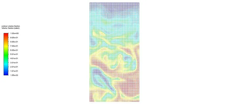 |
 |
| 300 | 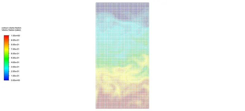 |
 |
| 400 | 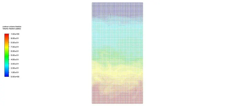 |
 |
| 450 | 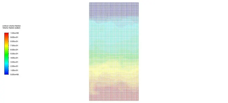 |
 |
| 500 | 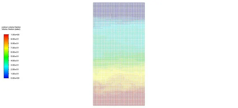 |
 |
Observation:
According to the grid independence test, we can observe that the normal mesh size(0.5mm) does not have that smooth flow, but arrives at the final settling of the phases with less simulation time, whereas, the finer mesh size(0.25mm) having a smooth flow and it takes time to settle down with more accuracy in the flow for the same time steps as given for normal mesh size.
Simulation for Water and Customised fluid(Density = 400 kg/m3, Viscosity = 0.001 kg/m-s):
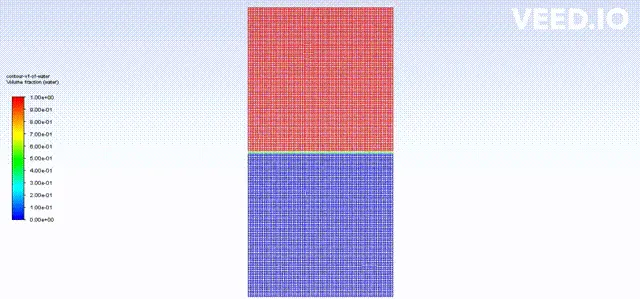
The following is the simulation of a relatively higher-density fluid in comparison to the air, patched with the water medium.
Observation:
The flow of the fluid under gravity is comparatively slow with the previous simulation since it is of higher density compared to air. Also, the formation of many vortices during the flow is evident which is not the case prior.
Atwood Number:
Atwood number is a dimensionless number and an important term in Rayleigh Taylor instability and Richtmyer-Meshkov Instability in order to find the penetration distance of the higher-density fluid into the lower one under the influence of acceleration in any form.
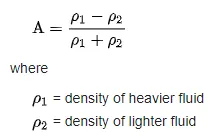
In here for the first case, the density of air is 1.225kg/m3 and water is approximately 1000kg/m3. So the Atwood number is 0.9975, whereas for the second case wherein the customized fluid has the density of 400kg/m3 the Atwood number value is 0.4285, thus we can infer that the penetration is more in the 1st case as it is evident from the test case.
Source: