Week 5 - Rayleigh Taylor Instability

Aim :

To find out Rayleigh Taylor Instability

Theory:

1. CFD and Rayleigh-Taylor Waves: A Simplified Approach

Simulating real-world mixing involving Rayleigh-Taylor (RT) waves in CFD software requires a balance between accuracy and computational cost. While the full mathematical analysis of RT waves exists, it's too complex for everyday CFD simulations.

To bridge this gap, practical CFD models adopt simplified approaches based on the core principles of RT waves. These models capture the essential physics using less demanding mathematical formulations. Think of it as a streamlined version focusing on the crucial aspects of RT instability relevant to the specific simulation.

Furthermore, these models employ techniques like adaptive meshing and interface tracking to maintain accuracy and efficiency. Adaptive meshing refines the grid in areas where RT waves are most prominent, while interface tracking methods follow the movement of the fluid boundary as the instability progresses.

In essence, CFD models leverage the knowledge of RT waves but adapt it for practical use by simplifying the math, focusing on key features, and employing efficient computational techniques.

1. Beyond Rayleigh-Taylor: A Family of Instability Phenomena

   While the Rayleigh-Taylor instability (RTI) is a fundamental concept, several related instabilities share similar characteristics.

   • Practical CFD Models: These models, often rooted in the mathematical analysis of waves associated with RTI (RT waves), are used in practical computational fluid dynamics (CFD) simulations.
   • Richtmyer-Meshkov Instability (RMI): Similar to RTI, RMI deals with mixing of fluids with different densities. However, RMI is triggered by a sudden acceleration, like a shockwave, while RTI involves a more gradual, steady force.
   • Kelvin-Helmholtz Instability: This instability arises when different fluid layers move at different speeds (velocity shear). When wind blows over water, it causes ripples to appear on the surface.
   • Plateau-Rayleigh Instability: This instability focuses on the tendency of liquids to minimize their surface area. It plays a role in the breakup of a continuous liquid stream into smaller droplets, relevant to specific ink technologies.

Richtmyer-Meshkov Instability:

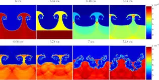
The Richtmyer-Meshkov instability (RMI) arises when a sharp interface separates fluids of contrasting densities, and this interface is subjected to a sudden acceleration. This acceleration, often caused by a shockwave passage, disrupts the equilibrium. Initially, small perturbations at the interface begin to grow linearly with time. However, as the instability progresses, a nonlinear regime takes hold. This regime is characterized by the formation of characteristic structures: bubbles if a lighter fluid penetrates a heavier one, and spikes if the opposite occurs. Ultimately, the instability reaches a chaotic state where the interface breaks down completely, leading to turbulent mixing of the two fluids.

RMI can be understood as the impulsive limit of the Rayleigh-Taylor instability (RTI). While both instabilities deal with interfacial mixing due to density differences, RTI operates under steady acceleration, whereas RMI involves a sudden, impulsive event.

• Fluid shearing triggers instability.

  Kelvin-Helmholtz instability arises when layers of a single fluid or different fluids move at different speeds (velocity shear). Imagine wind blowing over water; this is a classic example. The instability creates waves on the fluid surface, like ripples on water.

  Beyond Water: A Widespread Phenomenon

  This instability isn't limited to water surfaces. We can see its effects in clouds, ocean currents, Saturn's rings, Jupiter's Great Red Spot, and even the Sun's corona.

  Nature's Sculpting Tool:

  Kelvin-Helmholtz instability is a fundamental force shaping fluid motions across nature. From ocean waves to atmospheric clouds, it plays a crucial role in creating some of Earth's most familiar structures. By studying and modeling this instability, we gain a deeper understanding of the natural world.

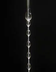
• Liquids tend to naturally form shapes that minimize their surface area, thanks to a property called surface tension. This principle is key to understanding an instability known as the Plateau-Rayleigh instability (often shortened to Rayleigh instability). This phenomenon describes how a continuous stream of liquid can break up into smaller droplets.

  The Rayleigh instability plays a significant role in fluid dynamics, particularly in the study of fluid fragmentation. It's also relevant to a specific type of ink technology where a liquid stream is disrupted to form a series of droplets. Recent research has focused on understanding the final shape (pinching profile) that forms during this instability, using similar approaches to those employed in studying other aspects of the phenomenon.

2.

1. Setting up geometry:

Creating two surfaces as air and water

Share the surfaces( Share Topology)

• Create 2 rectangles of size 20 x 20 mm, the lower one for air and the upper one for water.
• Create conformal mesh to have common interface between 2 interface & to share information.

2. Meshing the Geometry :

Baseline mesh: Create a baseline mesh of 0.5 mm.

3. Fluent setup :

Setting up physics :

Creating contour

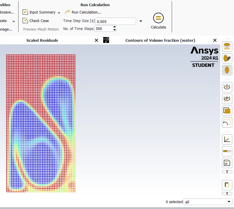
A. For mesh size of 0.5mm

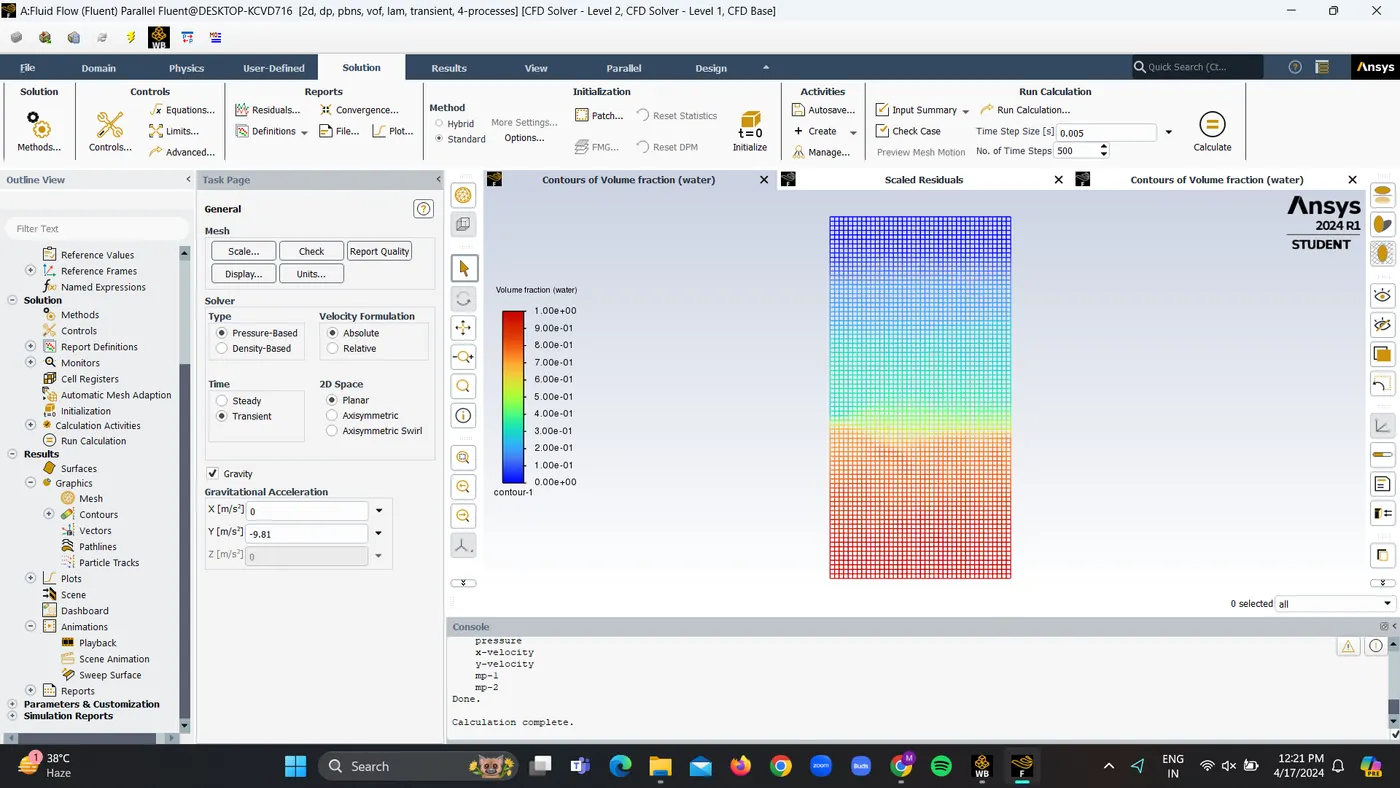
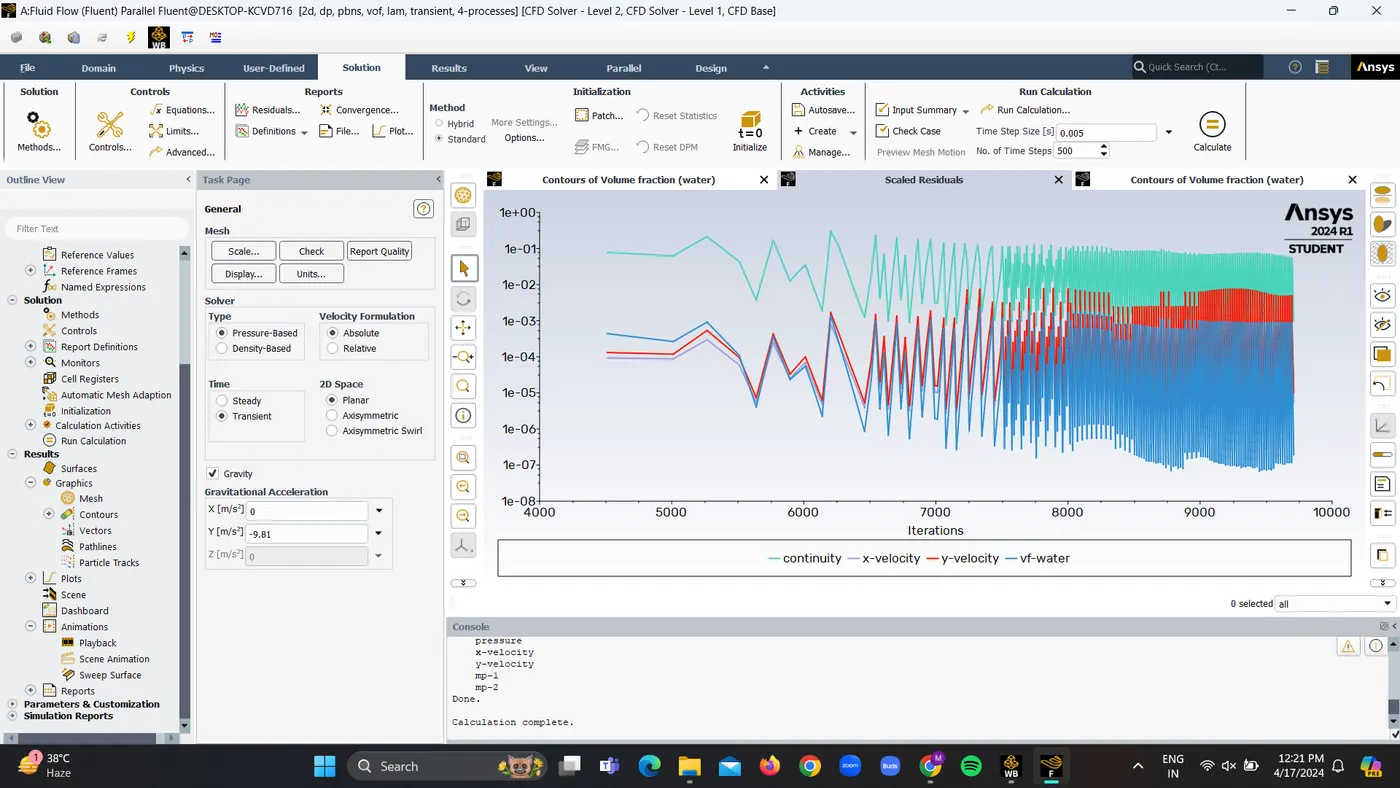
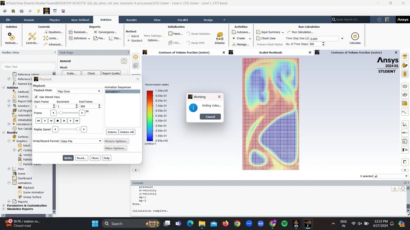
Link to the animation file:

https://drive.google.com/drive/folders/12CUPXDGY6zLa3VY4yDBwZQ6UciPeJI1w?usp=sharing

B. For mesh size of 0.3mm

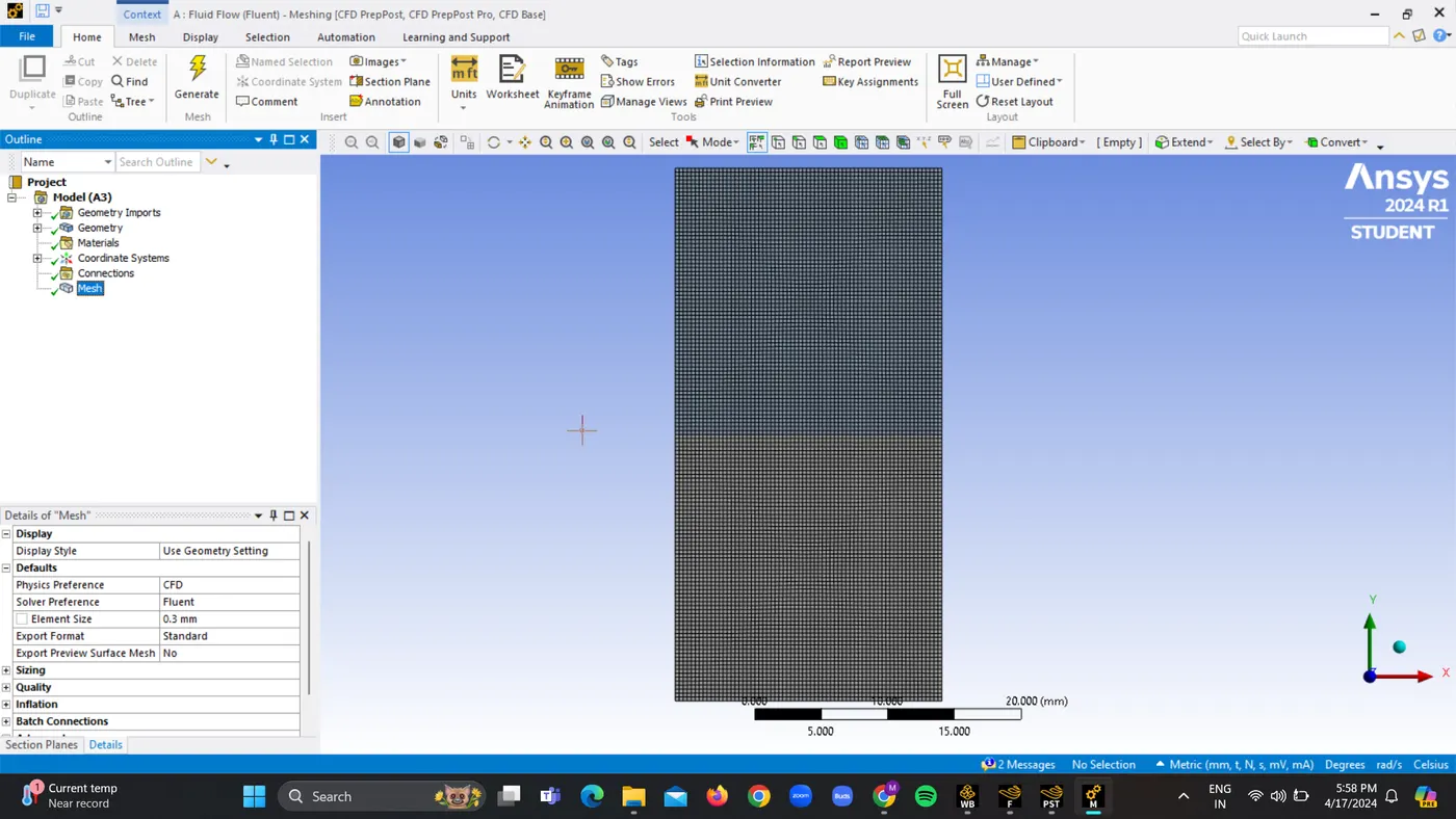
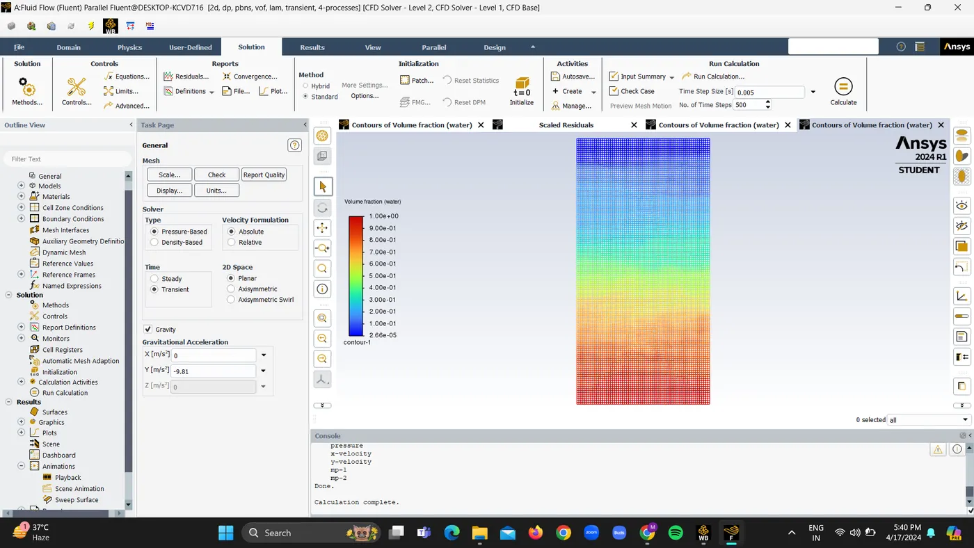
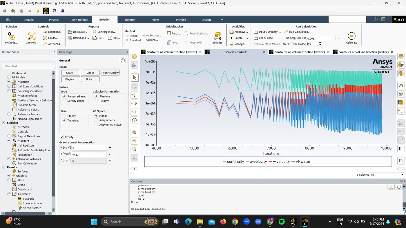
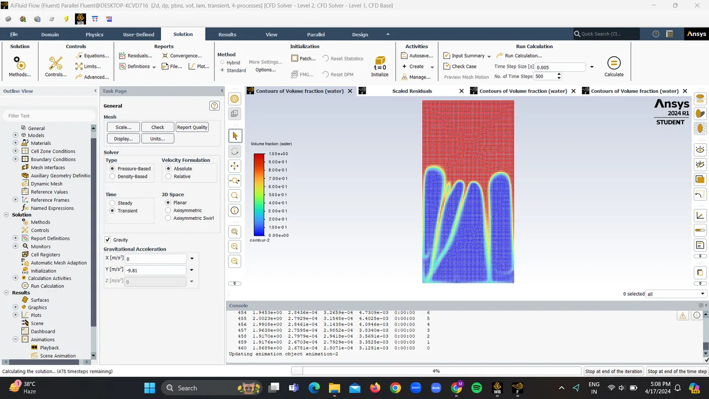
Link:

https://drive.google.com/file/d/12YufXRNCxhV6l5B4D-JD_ND3YPWyA3hc/view?usp=sharing

3. Run one more simulation with water and user-defined material (density = 400 kg/m3, viscosity = 0.001 kg/ms) for a refined mesh of 0.3mm.

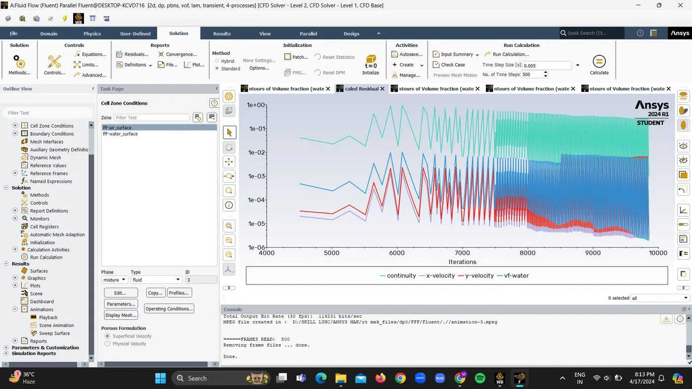
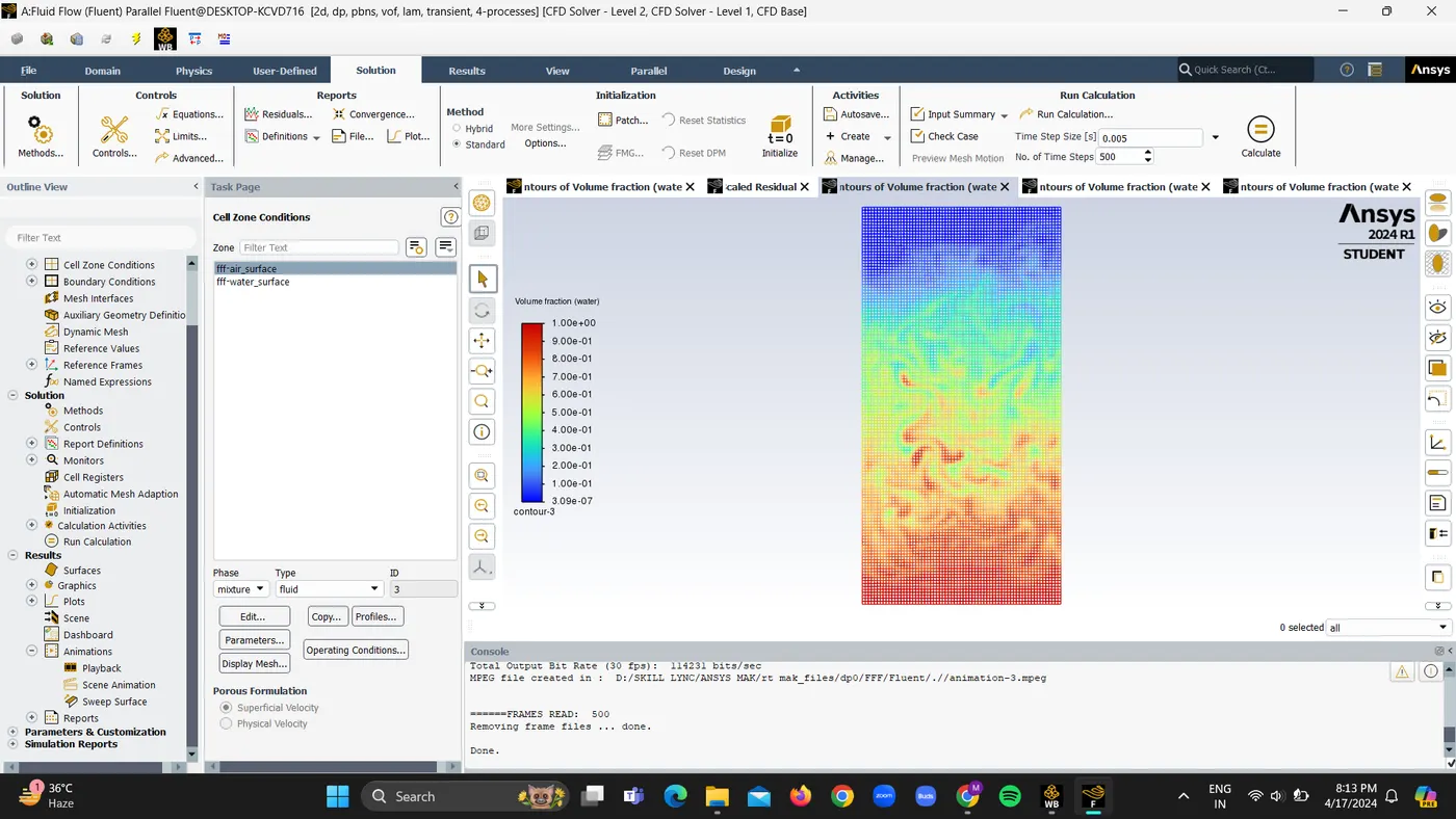
Link:

https://drive.google.com/file/d/135oAyGeoRmGSmSnjEvVNzBqERioLB07-/view?usp=sharing

4. Atwood Number and Instability Behavior:

The Atwood number (At) is a measure of the density difference between two fluids:

where:

Density of heavier fluid is

Density of lighter fluid is

a:

Density of water d1= 998.2 kg/m3

Density of air d2= 1.225 kg/m3

then atwood number be A= (998.2 -1.225)/(998.2 + 1.225)

A = 0.9975

b:

Density of water d1= 998.2 kg/m3

Density of user defined material d2= 400 kg/m3

A= (998.2 - 400)/(998.2 + 400) = 0.427

A=0.427

a: Air-Water (At = 0.997):

• High Atwood number indicates a significant density difference.
• The instability will grow rapidly with well-defined fingers and spikes due to the strong buoyancy force.

b: Water-User Defined Material (At = 0.427):

• Lower Atwood number indicates a smaller density difference.
• The instability growth will be slower with less pronounced fingers and spikes compared to the Air-Water case.
• The user-defined material being denser than Air but less dense than Water will result in a less vigorous instability development.

By comparing the Atwood numbers, we can predict the relative intensity of the RT instability in each case. A higher Atwood number leads to a more pronounced and faster-growing instability due to the stronger buoyant force driving the lighter fluid into the heavier one.