Week 5 - Rayleigh Taylor Instability

Aim:The aim to understand the Rayleigh Taylor Instability phenomena and how it take place.

Objective:

• Some practical CFD models that have been based on mathematical analysis of Rayleigh Taylor Waves.
• Explain how these mathematical modals have been adapted for CFD calculations.
• Perfrom the Rayleigh Taylor Instability simulation for 2 different mesh size with the base mesh being 0.5 mm. Compare the results by showing animations.
• Explain why a steady-state approach might not be suitable for these types of simulation.
• Run one more simulation with water and user-defined material(density=400kg/m^3,viscosity=0.001 kg/m-s)for refined mesh.
• Defined ehe atwood Number. Find out the Atwood number for both the cases and explain how the variation in Atwood number in the above two cases affect the behavior of the instability.

Rayleigh Taylor instability:

• From the newtons law of viscosity, wee know that even the fluid cannot resist the slightest shear force. Density is one of the main property of fluid which the shear force can incorporate with it.
• Depending upon the density we have lighter fluid like water etc and fluid like mercury,oil,honey etc.
• Rayleigh observed that when two liquids i.e lighter and heavier fluid are mixed together where the deser fluid is top on the lighter fluid,due to the gravity and the density variation the interface of liquid is not stable.(i.e) water suspended on the oil.
• So, the instability of the interface between the different densites of fluid when the lighter fluid is accelerated towards the heavier fluid is knowns as Rayleigh Taylors instability.

Richtmyer-Meshov instability:

The Richmyer-Meshkov instability(RMI) occurs when two fluids of different density are impulsively accelerated. Normally this is by the passage of shock wave. The development of the instability begins with small amplitude perturbations of the instability grow linearly with time. This is followed by a nonlinear regime with bubbles appearing in the case of a light fluid penetrating a heavy fluid, and with spikes appearing in the case of heavy fluid penetrating a light fluid. A chaotic regime eventually is reached and two fluids mix. This instability can be considered the impulsive-acceleration limit of the Rayleigh-Taylor instability.

Kelvin-Helmholtz instability:

The kelvin-Helmholtz instability can occur when there is velocity shear in single continuous fluid, or where there is velocity differnece across the interface between two fluids, An example is a wind blowing over water: The instability manifests in waves on the water surface.

Plateau-Rayleigh instability:

The Plateau-Rayleigh instability, often just called Rayleigh instability, explains why and how a falling stream of fluid breaks up into smaller packets with the same volume but less surface area. It is related to the Rayleigh-Taylor instability and is part of great branch of fluid dynamics aoncerned with fluid thread breakup.

Practical CFD models

SPH method(Smoother particle hydrodynamics):

Smoothed-particle hydrodynamics (SPH) is a computational method used for simulatind the mechanics of continuum media, such as solid mechanics and fluid flows. Smooth particle hydrodynamics is being increasingly used to model fluid motion as well. This is due to several benfits over traditional grid-base techniques. First, SPH guarantes conservation of mass without extra computation since the particle themselves represent mass. Second, SPH computes pressure from weighted contributions of neighboring particles rather than by solving linear system of equations. Finally, unlike grid-based techniques, which must track fluid boundaries, SPH creat afree surface for two-phase interacting fluids directly since the particles represent the denser fluid and space represents the lighter fluid.

Single-fluid mode:

A typical approah used for the analysis of two-phase flows is a mixture model, i.e. the individual fluid phases are assumed to behave as a flowing mixture described in terms of mixture properties. The applied single-fluid model is a five-equation model consisting of the mass, momntum and energy equtions for a vapor/liquid mixture, and two equations describing the formation and growt of liquid phase.

Two-fluid mode:

In the two-fluid model, seperate sets of the governing equtions for the vapor and liquid phases have been used. The interaction between the droplets and the heat exchange between the liquid phase and the solid boundary are not modelled here as well. Additionally, the velocity slip between vapor and liquid phase is in this model taken into account.

Turbulence model:

Turbulence model are needed to predict the average mixing behaviour in flow that are on average one or two-dimensional. The approach to the construction of tile turbulence model is guided by the experimental behaviour. The equtions governing turbulent flow can only be solved directly for simple cases of flow. For most real life turbulent flows, CFD simulation use turbulent models to predict the evolution of turbulence. These turbulence models are simplified constitutive equations that predict the statistical evolution of turbulent flows.

Geometry:

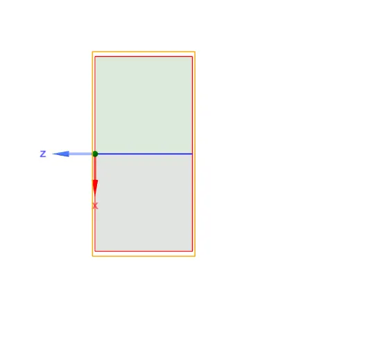
For our project, we consider a simple 2D geometry.

• We draw 2 squres one above the other with a length of 20mm.
• Then naming the below squre as air and above square as water in 2 different components.
• Share the topology for a perfect intersection between both surfaces.

Mesh:

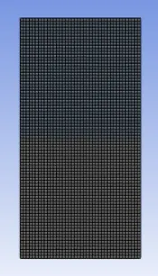
• In the mesh tree to open the mesh option change the element size to 0.5m .

SetUp:

Solver type                               Pressure -Based

Velocity Formulation                Absolute

Time                                         unstedy

                                                Viscous model:Laminar

Models                                     Multiphase:Volume of fluid                          

                                                               :Implicit formulation

                                                                :2 Phases

Material                                    Fluid type:Air

                                                              :Water Liquid

Cell zones                                  Fluid type:Air

                                                               :Water

Boudaries                                   Standard

Reference Values                         Standard

Initilization                                  Standard

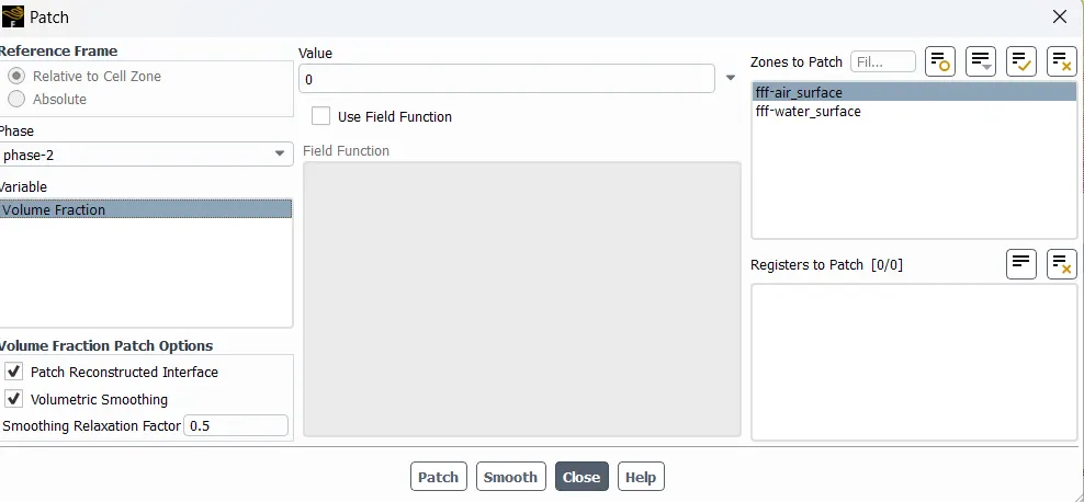
Patch                                          Water-surface (1 value of volume fraction of water)

                                                  Air-surface (0 value of volume fraction of water) 

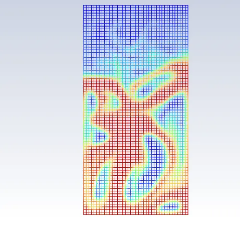
Case 1:

Element Size                            0.5mm

Number of elements                  3200

Density of primery fluid             Air(1.225 kg/m^3)

Density of secondary fluid          Water(998.2kg/m^3)

Time steps size                         0.005

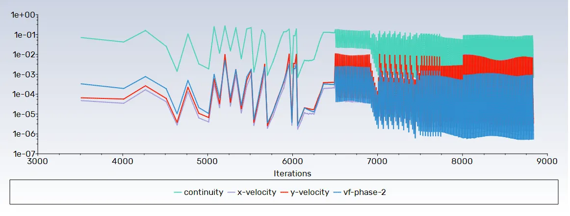
Number of iterations                  500

       

                                 

 

 Animation file:

 https://drive.google.com/file/d/1BqBcvMfl6T1vsNpZ19d2CO8LsytKyKJv/view?usp=sharing

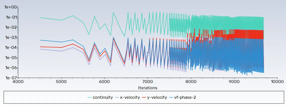
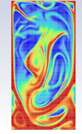
 Case 2:

Element Size                            0.2mm

Number of elements                  20000

Density of primery fluid             Air(1.225 kg/m^3)

Density of secondary fluid          Water(998.2kg/m^3)

Time steps size                         0.005

Number of iterations                  500

 

Animation Flie:

https://drive.google.com/file/d/1tVBR4Tn3Qm29lwRRuiWSu3Mlpx1T5rz2/view?usp=sharing

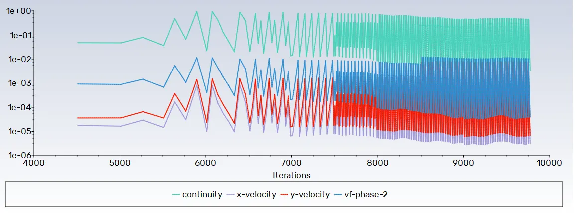
Case 3:

Element Size                            0.2mm

Number of elements                  20000

Density of primery fluid             Air(400 kg/m^3)

Density of secondary fluid          Water(998.2 kg/m^3)

Time steps size                         0.005

Number of iterations                  500

 

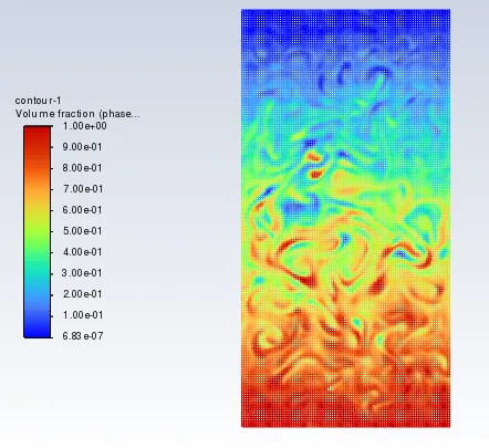
Animation Flie:

https://drive.google.com/file/d/1zBNza4go2jRv8faLngyPVLJJq6rIinmU/view?usp=sharing

Observation:

• The finer mesh capatures the instability better than the coarse mesh but it takes more time for the heavier to settle down.
• The computational time is also increased for fine mesh but the result obtained having better accuracy.
• The steady state simulation is perfromed if we are concerned more about the final state results or the equilibirium state, in RT instability CFD model we are more concerned to learn about the transition of the irregularities that start developing when we pour the high density fluid upon the low density fluid under the effect of gravity and we want to know how the interface collapses as a function of time so in this case Transient state is more suitable over the stedy state.

Atwood number:

The Atwood number (A) is dimensionless number in fluid dynamics used in the study of hydrodynamic instabilities in density stratified flows. It is a dimensionless density ratio defined as:

A=ρ1-ρ2/ρ1+ρ2

ρ1=Density of heavier fluid.

ρ2=Density of lighter fluid.

Conclusion:

• For A close to 0, RT instability flows take the from of symmetric "fingers" of fluid; for A close to 1, the much lighter fluid "below" the heavier fluid takes the from of larger bubble-like plumes.
• Atwood number is an important parameter in the study of Rayleigh-Taylor instability and Richtmyer- Meshkov instability. In Rayleigh-taylor instability, the penetration distance of heavy fluid bubble into the light fluid is function of acceleration time scale,A.f.t^2
• Where g is the gravitational acceleration and t is the time.
• For case1: Atwood number= (998.2-1.225)/(998.2+1.225)=0.9975
• For case2: Atwood number=(998.2-400)/(998.2+400)=0.4278.
• Therfore, penetration distance of heavy bublle A.g.t^2 in case 1 whould be higher, as it is directly prpotional to A(Atwood number).