Week 5 - Rayleigh Taylor Instability
Objectives -
1. To explain practical CFD models that have been based on the mathematical analysis of Rayleigh Taylor waves.
2. To perform Rayleigh Taylor instability simulation for 2 different mesh sizes and compare results showign animations.
3. To run another simulation with water and user-defined material with given specifications for refined mesh.
4. Define the Atwood number and explain how the variation in Atwood number in the above two cases affect the behaviour of the instability.
Theory -
When the lighter fluid is pushing the heavier fluid, RT instability—the instability of an interface between two fluids of differing densities—occurs. A common example of Rayleigh-Taylor instability is the suspension of water, a heavier fluid, over oil, a lighter fluid. This instability may be modelled by two immiscible fluid layers that are perfectly plane-parallel to one another, with the more dense layer sitting on top of the less dense layer and both being subject to gravity. If a volume of heavier fluid is pushed below and an equivalent volume of lighter fluid is displaced upward, the equilibrium is unstable to any perturbations or disturbances of the interface because the potential energy of the configuration is lower than the starting condition.
<!-- [if !supportLineBreakNewLine]-->
<!--[endif]-->
There are number of mathematical models for the analysis of RT waves-
1. Perturbation Models-
1.1 Haan’s second order analysis and saturation model-
An expansion of the flow equations provided the expression for the early nonlinear evolution (Ingraham, 1954, Jacobs and Catton, 1988a,b and references therein). A second order analysis by Haan (1991) was constructed for an interface between two materials in an imploding ICF capsule. For a slightly perturbed interface, an expansion was carried out in spherical harmonics to derive a second order mode-coupling equation.
1.2 Third order non-linearity-
A self-modulation of a primary mode produced by the third-order nonlinearity is a mechanism for deviation from the linear growth (Nishihara and Ikegawa, 1999). Motivated by the experimental data collected from the Nova laser system, Wood-Vasey et al. (2000) explored the amplitude saturation model of Haan (1989) and a 3rd order perturbation theory expansion of Jacobs and Catton (1988a). Based on the superposition of modes, Ikegawa and Nishihara (2003) developed thirdorder nonlinear theories that describe continuous transition from the linear to the weakly nonlinear growths of the classical RTI and the ablative RTI.
<!-- [if !supportLineBreakNewLine]-->
<!--[endif]-->
1.3 The Vandenboomgaerde-Gauthier-Mugler model-
Vandenboomgaerde, Gauthier, and Mugler (2002) advanced a simplified perturbation theory for nonlinear regime of a multimode RMI. The authors proposed a way to simplify and accelerate the computation for the perturbation theory in the weakly nonlinear RMI. In the standard approach, expansions appear to be series in time. The authors build accurate approximations by retaining the most secular terms, which are these with the largest unbounded part (Nayfeh, 1973, Bender and Orszag, 1978). The advantage of this approach is that computations for multimode interfaces become tractable.
1.4 Kelvin–Helmholtz (KH) instability-
In the classic understanding of the Kelvin-Helmholtz (KH) instability, wave perturbations of a two-layer shear flow gradually develop into billows and finally result in vertical mixing. The instability, however, can also be seen as a boundary-value issue. In such a framework, there is a situation upstream in which a lighter fluid flows over a denser fluid, and wave disturbances build downstream until finally overturning some distance from the place of origin. This flow demonstrates instability in space and is periodic in time, the opposite of the conventional issue. A natural example is when a warmer river empties into a lake or reservoir that is cooler.
1.5 Richtmyer-Meshkov instability-
When the acceleration is impulsive, as that from a shock wave, the RM instability may be thought of as a specific example of the RT instability. When a shock wave interacts with an interface separating two distinct fluids, the Richtmyer-Meshkov instability occurs. It covers a wide range of Mach numbers and integrates compressible processes like shock interaction and refraction with hydrodynamic instability like nonlinear development and eventual transition to turbulence.
1.6 Plateau-Rayleigh instability-
We will now discuss an effect that is frequently noticed wherever a thin liquid thread is flowing, such as from a tap. The liquid's thread will be steady for a while until it inevitably breaks down into individual droplets. Plateau-Rayleigh instability is the name given to this phenomenon. Surface tension produces strong forces that act on a fluid column. When the surface area is reduced, these can also be decreased. A liquid column will therefore have a propensity to break up into individual droplets. The theory of the Plateau-Rayleigh instability phenomena has several real-world applications. In order to ensure proper disintegration of a fluid jet into droplets, liquid dispensers, inkjet printers, and similar spotting systems are intended to produce perturbations (either by means of mechanical oscillations or thermally). Consider the fact that raindrops fall as droplets rather than as thin cylinders of water as an example of an everyday occurrence. Naturally, this idea is heavily utilised in droplet microfluidics to produce tiny droplets. Another significant area of use for the instability is the disintegration of thin coatings of viscous fluids, such as glues or paints, on wires and flat surfaces.
Solving and Modelling Approach -
Modelling -
1. First I opened spaceclaim and choose xy plane as a modelling plane.
2. Then I created a square of 20mm X 20mm.
3. Then I created a surface by using 'Pull' tool.
4. After coming out of 'Pull' tool I moved this surface to a new component and named this component as Air.
5. Then I created another component after right clicking on the parent Design section and named it as Water.
6. Then I created another square of similar dimensions of 20 mm X 20 mm.
7. Then I created a surface by using 'Pull' tool.
8. It was necessary to ensure conformal mesh between these two surfaces therefore I went to 'Workbench' of spaceclaim and went to 'SharePrep'.
9. Then I closed Spaceclaim and started Mesh environment.
10. Then I generated baseline mesh with 0.5 mm mesh size.
11. Then I closed Mesh environment and started Setup with Double Precision and 8 parallel processes.
12. Then I selected 'Transient' time, enabled gravity and gave it as as -9.81m/s^2 in y-direction.
13. Then I went to Physics, we are not going to solve energy equation in this simulation therefore I ignored 'Energy' checkbox and went in 'Multiphase' under Model section of Setup environment.
14. There in Models option I selected Volume of Fluid and under Volume Fraction Parameters I chose Implicit Formulation.
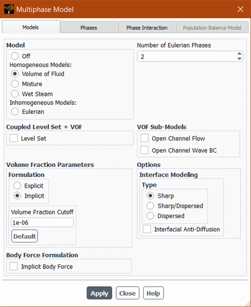
15. Then I went to Phases section under same Multiphase Model as shown below.
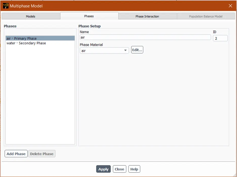
<>16. There I named Primary Phase as 'air' and Secondary Phase as 'Water'.
17. Then I closed Multiphase Model.
18. I went to Materials.
19. Since we had no water material therefore I went to Fluent Database and selected Water-Liquid material as shown below.
Note: For another simulation I needed to include User-Defined material for that as well I followed same steps.
20. Then I closed Material section.
21. Then I did Standard Initialization.
22. Then I went to 'Patch' as shown below.
23. Then I clicked on 'Volume Fraction' as you can see in the picture above and selected water_surface and gave '1' as Value and clicked on 'Patch'.
24. Then I clicked on air_surafce and gave '0' as value and clicked on 'Patch'.
25. Then I closed the Patch dialogue box.
26. Then to checked if it is patched properly I went to Contours and selected Phases, and selected the section on which this contour will be applied as shown below and clicked on Save/Display.
27. Then I went to Run Calculation and did the solution setup as per the instructions in the lecture.
28. Then I clicked on Run Calculation with 0.005 s as time step and 1500 no. of time steps.
<!--[endif]-->
Result -
Baseline Simulation contours -
<!--[endif]--> <!--[endif]--> <!--[endif]--> <!--[endif]-->
Refined Simulation Contour -
<!--[endif]-->
Water + User-Defined Material Refined Simulation Contour -
<!--[endif]-->
Simulation Videos-
Baseline Mesh 0.5 mm Simulation video-
https://drive.google.com/file/d/1tvVufzHIVJulV2YckK7WL2_SvUdKJxuS/view?usp=sharing
0.2 mm Simulation Video-
https://drive.google.com/file/d/1c6peq34lpE5gOg3zZs4LGcvlDnxVOsNp/view?usp=sharing
Water + User-Defined Material Simulation Video-
https://drive.google.com/file/d/1SaXzclU6vgnsUYANLhz3hd7v7r8tEC6k/view?usp=sharing
Why Steady-state approach might not be appropriate for this type of simulation?
This type of simulation directly involves lighter liquid at the bottom and heavier liquid at the top. In such scenario it is bound to happen that lighter liquid moves up and heavier liquid moves down over the period of time. Also, shock wave production occurs in RT instability as a result of the abrupt collapse of the horizontal plane between the dense and lighter fluid. And as a result, the time-dependent parameter, bubble and spike generation, occurs. So it really makes no sense to not consider the variable of time.
Atwood Number -
It is dimensionless number in fluid dynamics used in the study of hydrodynamic instabilities in density stratified flows.
`A = (ρ 1 − ρ 2)/(ρ 1 + ρ 2)`
<!-- [if !supportLineBreakNewLine]-->
<!--[endif]-->
rho1 = density of heavier fluid
rho2 = density of lighter fluid
Water & Air.......A = 0.997
Water & User-Defined Material.......A = 0.427
Effect of Atwood Number on behaviour of the instability -
When analysing rayleigh-tayor instability and richmyer-mechkow instability, the atwood number is a crucial factor. In RTI, where g is the gravitational acceleration and t is the time, the penetration distance of heavy fluid bubbles into the light fluid is a function of acceleration time scale.