Week 5 - Rayleigh Taylor Instability

AIM: To conduct the Rayleigh Taylor CFD simulation.

Rayleigh-Taylor:

The Rayleigh-Taylor instability is a fluid dynamics phenomenon that occurs at the interface between two fluids of different densities when subjected to a gravitational field. It leads to the mixing and interpenetration of the two fluids. This instability arises due to the competition between the buoyant force and the surface tension or pressure effects at the interface.

Here is how it works:

1. Initial Configuration: Imagine you have two fluids, often referred to as the "heavy" fluid and the "light" fluid. The heavy fluid is denser than the light fluid, and they are separated by an interface.
2. Gravity and Buoyancy: The heavier fluid exerts a gravitational force downward, and the lighter fluid exerts a lesser gravitational force upward. This leads to an instability, as the denser fluid wants to sink while the lighter fluid wants to rise.
3. Perturbations: If the interface between the two fluids is slightly perturbed, even by tiny ripples or waves, the heavier fluid will sink into the troughs of the perturbation, while the lighter fluid will rise into the crests. This amplifies the initial perturbation.
4. Amplification: As the interface evolves, the perturbations grow larger due to the gravitational forces causing the heavier fluid to accelerate and mix with the lighter fluid. The process continues, and the interface becomes more and more deformed.
5. Mixing: Eventually, the interface between the fluids becomes unstable, and significant mixing occurs. This is often observed as the heavier fluid penetrating into the lighter fluid in a complex and turbulent manner.

The Rayleigh-Taylor instability is of significant interest in various fields, including astrophysics, where it plays a role in the dynamics of stars, supernovae, and galaxy clusters, and in engineering, where it can affect processes such as inertial confinement fusion and fluid dynamics in nuclear reactors. It is important to note that other factors like viscosity, surface tension, and compressibility can influence the behaviour of the instability in different situations.

The opposite phenomenon, where a lighter fluid is on top of a denser fluid and the interface is perturbed, is known as the Kelvin-Helmholtz instability

PROCEDURE:

GEOMETRY:

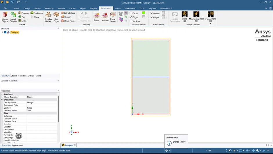
<!-- [if !supportLists]-->1.      <!--[endif]-->Draw 2 squares of length 20mm.

<!-- [if !supportLists]-->2.      <!--[endif]-->Then name the below square as air and above square as water in 2 different components.

<!-- [if !supportLists]-->3.      <!--[endif]-->Share the topology for a perfect intersection between both surfaces.

<!--[endif]-->

 

MESHING & SETUP:

CASE 1:

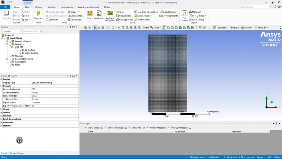
There is not much change to the fundamental mesh as it is a 2D object 

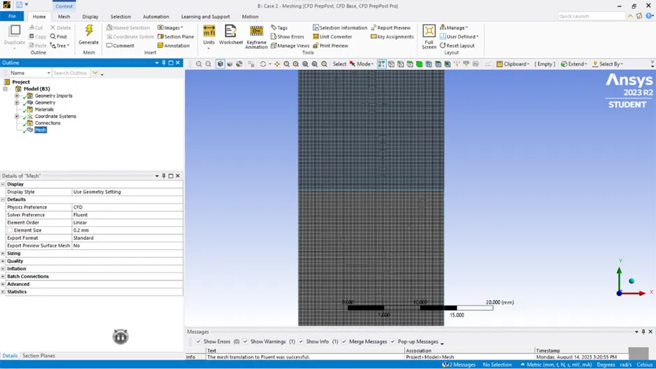
Overall Element size: 0.5mm (for case 1), 0.2mm (for case 2&3).

MESH OF 0.5MM

<!--[endif]-->

MESH OF 0.2MM

<!--[endif]-->

<!-- [if !supportLists]-->Ø  <!--[endif]-->For case 3, 0.2mm mesh is used.

SETUP:

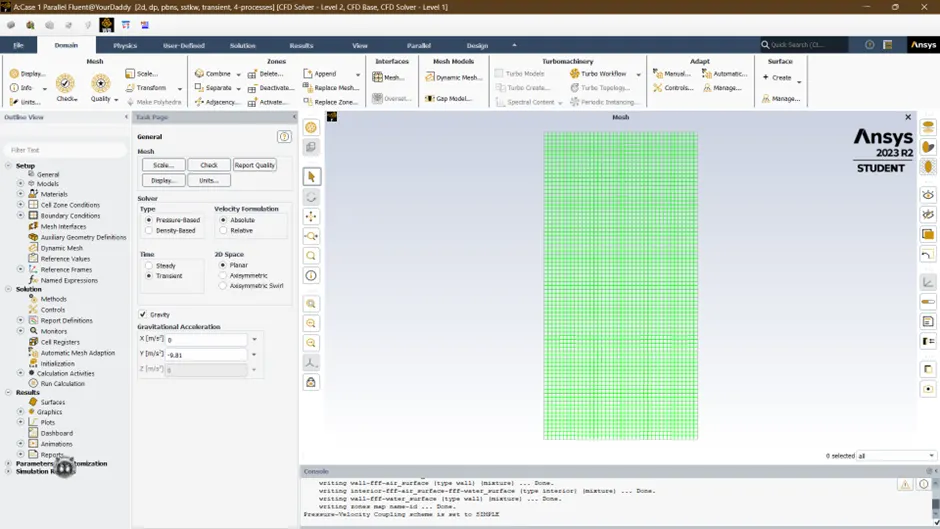
<!-- [if !supportLists]-->1.      <!--[endif]-->Solver- Pressure based and absolute velocity is used.

<!-- [if !supportLists]-->2.      <!--[endif]-->Transient state calculation.

<!-- [if !supportLists]-->3.      <!--[endif]-->Gravity is enabled in -ve Y-axis.

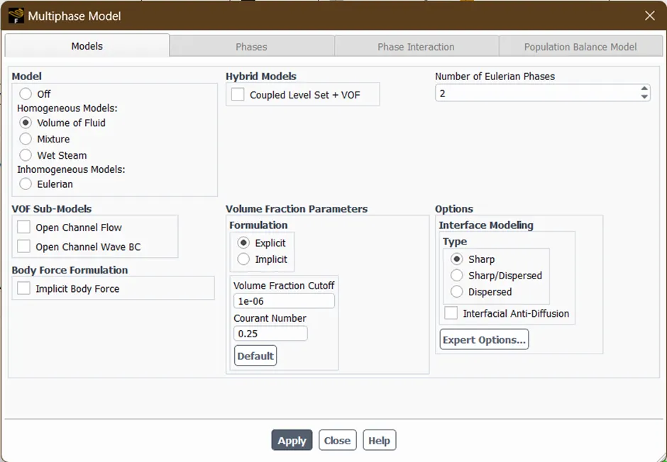
<!-- [if !supportLists]-->4.      <!--[endif]-->Multiphase model is turned on along with volume of fluid and number of Eulerian phases is chosen as 2. Accordingly, implicit scheme is selected.

<!-- [if !supportLists]-->5.      <!--[endif]-->Viscous model- Laminar is used

<!-- [if !supportLists]-->6.      <!--[endif]-->Patching of the volume of the two phases is performed.

<!-- [if !supportLists]-->7.      <!--[endif]-->Then patch the surfaces, “volume fraction of "1" is taken for water surface and "0" for air surface”.

<!-- [if !supportLists]-->8.      <!--[endif]--> Time step size (sec)= 0.005

<!-- [if !supportLists]-->9.      <!--[endif]--> No of Time steps: 1500

<!--[endif]-->

<!--[endif]-->

<!--[endif]-->

 

CASE 1

https://www.youtube.com/watch?v=n50rSDzv2o4

CASE 2

https://www.youtube.com/watch?v=xRiTQ7fibZQ

CASE 3

https://www.youtube.com/watch?v=3BiUI_Eo_FY

<!-- [if !supportLists]-->Ø  <!--[endif]-->Run the simulation with water and user-defined material (density = 400 kg/m³, viscosity = 0.001 kg/m-s) for refined mesh. i.e., Mesh size =0.2mm 

 

ATWOOD NUMBER:

A = ρ1- ρ2/ ρ1+ ρ2 (1)

where,

ρ1 = Density of heavier fluid `

ρ2 = Density of lighter fluid

Calculate the Atwood Number for Air-water RT instability

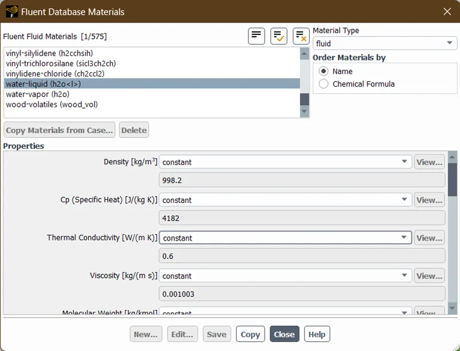
ρ1 = 998.2 kg/m3 (water density)

ρ2 = 1.225 kg/m3 (Air density)

put this value in equation 1 we get A = 0.9975

Calculate the Atwood Number for Water-UD material RT instability

ρ1 = 998.2 kg/m3 (Water density)

ρ2 = 400 kg/m3 (User defined material density)

put this value in equation 1 we get A=0.4278

The Atwood number close to “1”, which forms a larger bubble which is less symmetrical and it occurs very rapidly as shown in the animation.

The Atwood number close to “0”, which forms a bubble which is relatively symmetrical and the perturbations are linear for larger time as shown in the animation.

CONCLUSION:

• The finer mesh captures the instability better than the course mesh. But it takes more time for the heavier fluid to settle down as shown in the animation.
• Since the simulation involves capturing instabilities that are changing in an unpredictable manner as a function of time, the transient approach is preferred over the steady-state approach.
• The Atwood no validates the CFD simulation as it is observed. In the case of water and air mixing, bubble formation takes place, whereas in the other case no bubble takes place.