Week 5 - Rayleigh Taylor Instability

Aim:

To perform (i) simulations for two different sizes with base mesh 0.5 mm and for water-user defined material (density-400 `frac{kg}{m^3}` & viscosity-0.001  `frac{kg}{m-s}` (ii)a Study practical CFD model based on mathematical analysis of Rayleigh-Taylor waves and how the mathematical models has to implement in CFD calculations (iv)a study on importance of Atwood number for various cases that describes the Rayleigh-Taylor instability

Introduction:

Lord Rayleigh (1883) has published his classical treatment  entitled "Investigation of the Character of the Equilibrium of an Incompressible Fluid of Variable Density". It was motivated as an illustration of the theory of cirrus clouds but it is not specific for this case. The work describes the linear stability eigenvalue problem for incompressible fluids under gravity. The general stability criterion for incompressible inviscid fluids is discussed and particular perturbation solutions for exponential density variations are derived. It is remarkable that even a transcendental dispersion relation, describing the stability of exponential transition profiles, was already fairly completely analysed in this original work. Rayleigh was probably the first to pose the stability problem in a general manner and to recognize its principal significance for atmospheric stratifications. At his time, stable surface waves had already been well understood theoretically. The mathematical description of surface waves between superposed liquids of different densities may be largely due to Stokes (1847) . Some early observation of the density dependence of the oscillation period was apparently made by Benjamin Franklin (1762) , who compared the behavior of oil-water and air-water interfaces. In later works, some of the idealizations of the inviscid incompressible fluid model have been overcome. Schwarzschild (1905) has established the basic criterion for stability against convection in compressible atmospheres. Harrison (1908) included the effect of viscosity in the treatment of superposed fluid layers and Rayleigh (1916) could explain the onset of Boussinesq convection by including viscosity and thermal conductivity. Apart from these and other early studies of gravitational instabilities, the modern developments have started with the work of Taylor (1950). In a companion work by Taylor and Lewis , the basic physical importance of RT instabilities for accelerated fluid layers could first be demonstrated. The theoretically predicted instability growth rates proved in excellent agreement with laboratory experiments. Furthermore, the subsequent stage of rising upstanding gas columns could be observed. The rate of rise of these gas columns could be explained by similar laws as for underwater bubbles and for bubbles rising in cylindrical tubes. These findings have been highly influential for the future developments. In the succession of Taylor's work, the instability theory was rapidly developed in various directions to include, for instance, surface tension and viscosity, magnetic fields , spherical geometries , finite-amplitude perturbations, and bubble theories. There exist already excellent reviews of parts of the instability theory, especially those by Chandrasekhar  and by Birkhoff . Chandrasekhar's work gives an overview on the linear theory for incompressible continuous media. Birkhoff's report describes the principle instability problems in potential flow theory along with a discussion of possible solution methods for linear and nonlinear evolution. Unfortunately, the latter work has not been published and existing copies of the original manuscript are quite cumbersome for reading. The textbook of Drazin and Read represents another valuable introduction to hydrodynamic instabilities. However, there is only little overlap with the present RT problem, since this work has been largely devoted to the topics of thermal instabilities and shear flow instabilities.

 The instability of a heavy fluid layer supported by a light one is generally known as Rayleigh-Taylor (RT) instability. It can occur under gravity and, equivalently, under an acceleration of the fluid system in the direction toward the denser fluid. Even if an unstable equilibrium would be established, the instability evolution would be too fast for direct observation. However, the typical finger-like flow patterns can be nicely modeled, for instance, by Hele-Shaw cells consisting of thin sheets of viscous fluids inside the gap between two parallel glass plates.

 The first experiments by Lewis  have shown three subsequent stages in the evolution of an unstable air-water interface. The initial phase of exponential growth is followed, first, by a transition phase of bubble formation and then by an asymptotic stage of rising air columns. One should clearly distinguish between the instability problem, related to the initial phase, and the mixing problem, related to the asymptotic phase. In the instability problem, one is mainly concerned with the modification of instability growth rates by various physical effects. In contrast, the mixing problem is addressed to the penetration of perturbation fronts through the liquid.

 Another series of experiments by Emmons et al. has largely confirmed these findings. In addition, the effect of surface tension was investigated. Theoretically, it leads to stabilization of perturbations with wavenumbers larger than the cutoff , where ρ denotes the density and T the surface tension. The experimental results have indicated the trend toward reduced growth rates close to the cutoff, although complete stabilization was not observed. This lack of agreement was explained in part with inaccuracies in the determination of the initial amplitude and in part with nonlinearities. The experiment was reconsidered by Cole and Tankin with improved accuracy, but with about the same cutoff behavior.

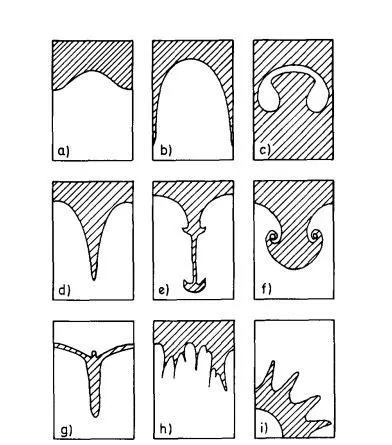
 More advanced stages of intermixing have been observed by Read and by Dikarev and Zatsepin  in the RT case. Similar experiments have been performed by Andronov et al. in the Richtmyer-Meshkov case. Although a unique picture of mixing layers has not yet emerged, a trend toward larger bubble structures has been clearly observed. The experiments of Read have even indicated a simple similarity law for mixing layer growth in proportion to the acceleration distance of the fluid system.  The heavy (light) fluid is represented by shaded (unshaded) regions and the kinematical acceleration is directed vertically upward in (a-h) or radially inward in (i). Normal mode perturbations of the horizontal equilibrium surface give rise to sinusoidal surface modulations as represented in (a). The fluid interchange decreases the potential energy content of the system which is the cause of instability. The further upward motion of the lighter fluid assumes the form of rising gas bubbles with an approximately steady shape as illustrated in (b). For comparison, the evolution of a closed, initially spherical bubble is also shown in (c). These horseshoelike deformations are based on incompressible inviscid fluid dynamics. Experimental observations of underwater bubbles have also indicated the formation of a turbulent wake. Typical features of the falling heavy fluid are represented in (d-g). In a low-density gas, the fluid particles can closely approach the stage of free fall. A corresponding contraction of the downward flow gives rise to needle-shaped spikes as shown in (d). When the flow resistance of the lighter fluid becomesimportant, as in (e), broadening of the spike tips is observed along with the formation of mushroom-like vortex motions. These additional structures are commonly attributed to secondary shear flow instabilities. The pronounced differences between bubbles and spikes disappear for fluids with nearly equal densities . Corresponding bubble-spike pairs can be recognized in (f). Anti-spikes, of the form shown in (g), have been observed in fluid simulations  at the stable rear side of an accelerated thin foil. They have been explained theoretically as a result of colliding jets at a cusp point singularity in the surface equation of thin layers . The advanced stage of intermixing  gives rise to much more complicated flow patterns as illustrated in (h). RT instabilities are also often encountered in spherical geometries (i). For instance, implosions of inertial confinement fusion pellets are subject to outside surface instabilities during acceleration and to inside cavity instabilities during deceleration. Over the past decades, it also became obvious that RT instabilities would play an important role in many different fields. Their control is of vital interest for a number of technological applications, in particular in inertial confinement fusion (ICF) devices . A number of experiments have demonstrated the physical significance of these instabilities in ICF [24-33]. In some cases, reduced growth rates, mostly attributed to ablative modifications, have been found. Other examples have been reported in geophysics, where some ionospheric phenomena, known as equatorial spread F bubbles, have been explained in the RT context . In astrophysics, certain chain-like globules (elephant trunks) in the interstellar medium show close resemblance with RT flow patterns . It is therefore believed that RT instabilities can occur in accelerated gas clouds, driven for instance by new-born stars  or supernova events. Other astrophysical RT instabilities have been discussed for magnetic field-supported accretion disks in neutron stars and for collapsing stellar cores due to an intense release of neutrinos.

 An elementary description of RT instability can be given in terms of potential flow theory. It provides a well-known framework for the study of surface modes and has been the basis of many classical stability results. Important aspects of this approach are that the most severe interfacial perturbations can be isolated by this model, giving usually an upper bound on instability growth.Furthermore, it pertains to nonlinear evolution in a relatively simple manner.Applications of potential flow theory. Firstly, the stability of a single plane interface is outlined, leading to the classical growth formula for the combined RT and KH instabilities. The analysis of a single unstable interface is then extended to layers of finite width where Taylor's free-surface model is presented.Theory a three-layer model, displaying essential features of accelerated foils and anti-mixing layers

RT instability marks only the onset of a complex interpenetration process, leading ultimately to the growth of mixing regions between neighboring fluids. On the other hand, the evolution of a free surface may be largely understood from first principles as an evolution of rising gas bubbles.a number of bubble models that have proved particularly successful in the prediction of bubble parameters. These are the spherical-flow model of Taylor, the single-mode model first discussed by Layzer, and the source-row model introduced by the present author. Finally, applications of bubble theory to buoyancy-driven mixing layers.Nonlinear perturbation theories of the RT instability have been intensively studied in the presence of surface tension.Free-surface bubbles may be classified according to their topology as open or closed ,Closed bubbles will be solved with the help of spherical bubble model,open bubbles will be solved with steady state model.The potential flow model, discussed so far, describes the motion of fluid layers with piecewise constant densities. In the following, we will consider incompressible fluids with continuous density variations. A basic difference arises from the possibility of vorticity generation in the presence of nonlinear pressure and density gradients. The evolution of these rotational modes and their relationship to the surface modes of potential flow theory is the main subject.We first introduce the nonlinear evolution equations for two-dimensional incompressible flow in an inhomogeneous medium..Incompressible flow model is one of the model for solving.Single Mode model is utilised for mixing motions in RT instability.

viscosity acts already in homogeneous fluids and it is responsible for the dissipation of kinetic energy on small spatial scales. This property is particularly important in boundary layer flows, in the evolution of homogeneous fluid turbulence, and in the present context, as a damping mechanism for fluid instabilities.the surface instabilities between two uniform fluid layers are examined in the presence of shear flow, buoyancy and viscosity.Viscous flow model  allows to determine finite maximum growth rate of the instabilities.RT instabilities in incompressible viscous fluids, including effects of surface tension and of variable fluid densities.

 The ideal fluid model provides a means for the investigation of the stability of compressible dissipationless fluids.Compressibility affects in an essential way the instability threshold,leading to Schwarzschild's stability criterion for convective instabilities.The ideal fluid model of RT-type instabilities concerns also several issues of more theoretical interest. These include for instance (i) the stability criterion for convective instabilities, (ii) its relationship to the energy principle for ideal fluids, (iii) dependences on special material equations (ideal gas approximation), and (iv) the role of compressibility for instability growth.

 The RT instability of ablatively accelerated foils is strongly influenced by mass ablation,heat flow, and inhomogeneities.For most applications, the ablation front can be regarded as a subsonic, approximately isobaric flow region. Within this region the instability evolution may be well described by an isobaric flow model.

Similar to Rayleigh-Taylor instability:

The instability of shock-accelerated interfaces has been studied theoretically by Richtmyer [8] and experimentally by Meshkov. It was found that the long-time evolution of Richtmyer-Meshkov instabilities can be well described by the model of an impulsive RT instability.The Richtmyer–Meshkov instability (RMI) occurs when two fluids of different density are impulsively accelerated. Normally this is by the passage of a shock wave. It describes constant velocity growth of initial surface corrugations.The RT instability is utlised for a variety of different acceleration laws, including the impulsive acceleration model of the Richtmyer-Meshkov instability.

 The Plateau–Rayleigh instability is named for Joseph Plateau and Lord Rayleigh. In 1873, Plateau found experimentally that a vertically falling stream of water will break up into drops if its length is greater than about 3.13 to 3.18 times its diameter, which he noted is close to`pi` . Later, Rayleigh showed theoretically that a vertically falling column of non-viscous liquid with a circular cross-section should break up into drops if its length exceeded its circumference, which is indeed `pi` times its diameter.Plateau–Rayleigh instability explains why and how a falling stream of fluid breaks up into smaller packets with the same volume but less surface area.

 Hermann von Helmholtz in 1868. Helmholtz identified that "every perfect geometrically sharp edge by which a fluid flows must tear it asunder and establish a surface of separation".Following that work, collaborator William Thomson (later Lord Kelvin), developed a mathematical solution of linear instability whilst attempting to model the formation of ocean wind waves. In the early 1920s, Lewis Fry Richardson developed the concept that such shear instability would only form where shear overcame static stability due to stratification, encapsulated in the Richardson Number.The ideas of Kelvin-Helmholtz instabilities were applied to a range of stratified fluid applications.The Kelvin–Helmholtz instability (after Lord Kelvin and Hermann von Helmholtz) is a fluid instability that occurs when there is velocity shear in a single continuous fluid or a velocity difference across the interface between two fluids.

CFD Models based on Rayleigh taylor instability

1. Buoyancy drag model:It is valid for every Atwood number but limited to non-linear stages of the instability. The Buoyancy–Drag model is a simple model, based on ordinary differential equations, for estimating the growth of a turbulent mixing zone at an interface between fluids of different density due to Richtmyer–Meshkov and Rayleigh–Taylor instabilities. Small initial interface perturbations form “bubbles” of light fluid which penetrate the dense fluid and “spikes” of dense fluid which penetrate the light fluid.This model cannot deal with multiple mixing interfaces; cannot be easily extend to two or three dimensions, and as a rule, do not address demixing, also known as counter gradient transport i.e. reduction of total fluid masses within the mixing zone. To address the above problems, two-fluid (multi-fluid) models has to be used. 
2. Single Fluid variable density model(Besnard-Harlow-Rauenzahn):It is more advanced version of the single-fluid model. The BHR model is based upon the evolution equations arising from second-order correlations and gradient-diffusion approximations. Using a mass weighted-averaged decomposition, the original BHR model includes the full transport equation for the Reynold's stresses, turbulent mass-flux velocity, density fluctuations and turbulent kinetic energy dissipation rate.RM and RT instabilities determined a coefficients. It is valid for the compressible flow.
3. 3.K-ε turbulence model (two equation):In that respect, it should be mentioned that in the experiments we are interested in we only have access to the mixing-zone thickness, some mean flow quantities such as concentration or temperature. The behavior of these quantities are usually well reproduced, and sometimes better described, by simple K-ε models. The diffusion terms of the k and ε equations are handled in a coupled implicit manner while Rayleigh-Taylor source terms are discretized in an explicit way.Attempted to connect   and   which are the coefficients of the Rayleigh-Taylor source term in the k and ε equations.
4. K-L Turbulence model:In the k-L model is to use the turbulent length and kinetic energy scales to construct an eddy viscosity,. This viscosity is then used to compute the turbulent fluxes of species mass fraction, X and internal energy, e.It used three test problems to calibrate these parameters (three coefficients in the equation) independently: a shear layer growth KH test case, a constant g RT test case, and impulsive acceleration RM test case.

 Mathematical model adaptions for CFD calculations:

Naming some of the mathematical models of the Rayleigh-Taylor instability are (i)Double infinite fluid Taylor instability (ii)Finite thickness double interface fluid (iii)Fluid interface movement of finite thickness two-sided vacuum (iv)Variable density fluid layer (v)The Taylor instability of viscous fluids (vi)Ablation instability (vii)RT instability of magnetic field in MHD etc..,So the mathematical models means an Equations that  is developed based on the discretization scheme,boundary or initial conditions,type of the flow of the geometry these are the things we will give as an inputs to the cfd models(principles).By the solver,mathematically modelled problem is to be calculated a various parameters.Solver includes an algorithm,schemes for spatial discretisation and temporial.

Modelling: 

Geometry:

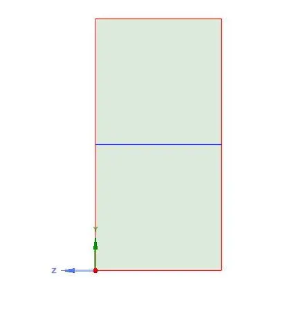
Spaceclaim is used to create initial volumes of air and water.Geometry of the fluid is square with the length and width of 20 and 20 mm.Two fluids share the information across the interfaces.

Meshing:

 

On the used 2D structure,we can see the meshing of the quadrilateral elements as a default.

	Element Size	Elements
Baseline Mesh	0.5 mm	3200
Medium size Mesh	0.35 mm	6498
Refined Mesh	0.245 mm	13448

 All the meshes described above are good element quality,skewness,aspect ratio and orthogonality

 Physics setup:

1. Pressure-based solver is used to mean this flow as incompressible flow.Velocity formulation, absolute is used to values entered are global reference coordinate system.
2. Transient time is used and 2D space is planar because our geometry looks like plane.

Why steate state approach is not suitable this type of simulation?

Instability at interface starts with small pertubations and grow linearly with time.if we do steady state approach equations will be changed it provides a result as how it looks like in a equilibrium (or) stable.pseudo transient at steady will somewhat approximate a transient but it cant able to capture the behaviour of a very small time step.Transient will shows the behaviour of instability as well steady state after the instability behaviour.

3. Rayleigh taylor instability will have a significant parameter called gravitational acceleration thas why provided the negative value of 9.81 m^2/s in the Y-direction under the gravity check box.
4. Selected a viscous model as laminar due to controlling the growth rate of pertubations.
5. Here we are using two fluids to model RTI.For that need to copy the two materials such as air and water from the fluent database.These two materials will present at material database.
6. VOF(Volume of fraction)Model is used under the multiphase flow.(The VOF model can model two or more immiscible fluids by solving a single set of momentum equations and tracking the volume fraction of each of the fluids throughout the domain. Typical applications include the prediction of jet breakup, the motion of large bubbles in a liquid, the motion of liquid after a dam break, and the steady or transient tracking of any liquid-gas interface.).Described the no of phases is 2.Sharp interface modelling is used,includes lagrangian methods with move meshes,front tracking,levelset,hybrid methods etc..,
7. Cellzones and boundaries defined automatically with good assumptions
8. On the solver,default solvers are used but transient formulation changed to bounded second order implicit to avoid the divergence
9. If we use multiphase flow,standard initialisation is used for patching the volume of fraction under the patch option.
10. Patching the air as 0 volume of fraction and water as 1.
11. Created the phases (or) volume of fraction contours  to view the behaviour of instability
12. Created the animation based on phases contour  by using solution animations option
13. Using the timestep size as 0.005s and 1000 timsteps and ran the simulation
14. Repeat the procedure for different mesh sizes.
15. For User Defined material on the step 5 we need to add one more step that water material is once again added with naming and have to change the density and viscosity and create it and on step 8 have to change the phase material under phases tab on the mutiphase flow task window.

Behaviour of Rayleigh-Taylor instability animation:

air-water interface

1.Base mesh 

2.Medium size Mesh

3.Refined Mesh 

Water-User defined material Interface

1.Refined mesh

Atwood Number:

The instability evolution between fluid layers of nearly the same density has been studied experimentally by Allred and Blount  and by Ratafia. The density dependence can be expressed by the so-called Atwood number leading to appreciably lower growth rates for fluids with nearly equal densities.The Atwood number (A) is a dimensionless number in fluid dynamics used in the study of hydrodynamic instabilities in density stratified flows. It is a dimensionless density ratio defined as

 A =`frac{underset(1)(rho)-underset(2)(rho)}{underset(1)(rho)+underset(2)(rho)}`

`underset(1)(rho)`-Density of heavier fluid

`underset(2)(rho)`-Density of lighter fluid

Moreover, the nonlinear evolution of the interface appears more symmetric, showing mushroom-like flow patterns in both fluids.For A close to 0, RT instability flows take the form of symmetric "fingers" of fluid; for A close to 1, the much lighter fluid "below" the heavier fluid takes the form of larger bubble-like plumes.

Atwood numbers for two cases (i) water-air (ii)water-userdefined material

 Case 1

A=`frac{998.2-1.225}{998.2+1.225}`=0.99754

 Case 2

A=`frac{998.2-400}{998.2+400}`=0.42783

Conclusion:

1. By decreasing the size of the mesh behaviour of instability shows the differences only at interfaces.volume of fraction  changes gradually from 1 at bottom to the 0 at the top .on baseline mesh occupying volume of fraction 0 is less when compared to refined mesh in the similar way volume of fraction 1 is also appeared.Refined mesh provides good detailing near the interface.
2. Atwood number near 1 shows the interface starts to deform in the bubble shapes.Atwood number 0.4278 shows the interface starts to deform like finger structure.
3. Atwood number near 1, low density fluid penetrate into higher density fluid in bubble shape where as penetrate of higher density fluid into low density fluid in the spike shape it is clearly visible.
4. Bubbles would be formed at Atwood number near 1 is big and small at atwood number 0.4278.
5. Time taken to became a stable or equilibrium based on atwood number,atwood number 0.4278 would take time (slow growth rates) compared to the atwood number near 1.
6. Atwood number would be significant for  growth rates,formation of bubbles,type of intial interference deformation.

References:

1. 1.A k-ε model for turbulent mixing in shock-tube flows induced by RayleighTaylor instability Serge Gauthier and Michel Bonneta)
2. The k-L turbulence model for describing buoyancy-driven fluid instabilities VINCENT P. CHIRAVALLE.
3. Buoyancy–Drag modelling of bubble and spike distances for single-shock Richtmyer–Meshkov mixing,PanelDavid L. Youngs, Ben Thornber.
4. Turbulence Transport Equations for Variable-Density Turbulence and Their Relationship to Two-Field Mode ,Didier Besnard,Francis H. Harlow ,Rick M. Rauenzahn ,Charles Zemac.
5. SOME MATHEMATICAL MODELS AND MATHEMATICAL ANALYSIS ABOUT RAYLEIGH-TAYLOR INSTABILITY,Boling Guo ,Binqiang Xie.
6. THEORY OF THE RAYLEIGH-TAYLOR INSTABILITY ,H.J. KULL.

Alternative Animation Links:

1.basemesh - https://drive.google.com/file/d/1QYNuEjoZh64OFW7w22va7qQxeBc_CxI_/view?usp=drive_link

2.medium size mesh-https://drive.google.com/file/d/1AG-lMScniZg9zaDScx_sWwfR2EFHuTGU/view?usp=drive_link

3.refined mesh-https://drive.google.com/file/d/1YV-4jGHURjSYQDxhB3PO9YPxjYwNGKLw/view?usp=drive_link

4.Udf -https://drive.google.com/file/d/1ez2TanijVPgEnk2iZM7WQK_kBE458_4_/view?usp=drive_link