Week 5 - Rayleigh Taylor Instability

RAYLEIGH TAYLOR INSTABILITY SIMULATION

AIM:

To perform the Ryleigh Taylor instability for differenr mesh sizes and also to compare the results obtained by changing the materials.

OBJECTIVE:

1.Perform Rayleigh Taylor Instability for Base mesh of 0.5 mm and run the simulation for both steady and transient cases.

2.To observe the animation results and to compare the effect mesh.

3.To run one another simulation with water and user defined material and to discuss and compare the results with the previous case.

4.To define the Atwood Number for both the cases and to compare the Instability behaviour for two cases.

5. Theory on some practical CFD models and mathematical analysis of Rayleigh Taylor waves.

Rayleigh–Taylor instability: The Rayleigh–Taylor instability, or RT instability (after Lord Rayleigh and G. I. Taylor), is an instability of an interface between two fluids of different densities which occurs when the lighter fluid is pushing the heavier fluid. Examples include the behavior of water suspended above oil in the gravity of Earth, mushroom clouds like those from volcanic eruptions and atmospheric nuclear explosions, supernova explosions in which expanding core gas is accelerated into denser shell gas, instabilities in plasma fusion reactors and inertial confinement fusion.

There are some practical CFD models that have been based on the mathematical analysis of Rayleigh Taylor waves:

1.Kelvin–Helmholtz instability: The Kelvin–Helmholtz instability (after Lord Kelvin and Hermann Von Helmholtz) can occur when there is velocity shear in a single continuous fluid, or where there is a velocity difference across the interface between two fluids.

An example is wind blowing over water: The instability manifests in waves on the water surface. More generally, clouds, the ocean, Saturn\'s bands,Jupiter\'s Red Spot, and the sun\'s corona show this instability.

The theory predicts the onset of instability and transition to turbulent flow in fluids of different densities moving at various speeds. Helmholtz studied the dynamics of two fluids of different densities when a small disturbance, such as a wave, was introduced at the boundary connecting the fluids.

For a continuously varying distribution of density and velocity (with the lighter layers uppermost, so that the fluid isRT-stable), the dynamics of the KH instability is described by the Taylor-Goldstein equation and its onset is given by the Richardson number Ri.

Typically the layer is unstable for Ri<0.25. These effects are common in cloud layers. The study of this instability is applicable in plasma physics, for example in inertial confinement fusion and the plasma - berryllium interface.

2.Richtmyer–Meshkov instability: The Richtmyer–Meshkov instability (RMI) occurs when two fluids of different density are impulsively accelerated. Normally this is by the passage of a shock wave. The development of the instability begins with small amplitude perturbations which initially grow linearly with time. This is followed by a nonlinear regime with bubbles appearing in the case of a light fluid penetrating a heavy fluid, and with spikes appearing in the case of a heavy fluid penetrating a light fluid. A chaotic regime eventually is reached and the two fluids mix. This instability can be considered the impulsive-acceleration limit of the Rayleigh-Taylor instability. Examples - During the implosion of an inertial confinement fusion target, the hot shell material surrounding the cold D-T fuel layer is shock-accelerated. This instability is also seen in Magnetized Target Fusion. Mixing of the shell material and fuel is not desired and efforts are made to minimize any tiny imperfections or irregularities which will be magnified by RMI.

Supersonic combustion in a Scramjet may benefit from RMI as the fuel-oxidants interface is enhanced by the breakup of the fuel into finer droplets. Also in studies of deflagration to detonation transition (DDT) processes show that RMI-induced flame acceleration can result in detonation.

3.Plateau–Rayleigh instability: The Plateau–Rayleigh instability, often just called the Rayleigh instability, explains why and how a falling stream of fluid breaks up into smaller packets with the same volume but less surface area. It is related to the Rayleigh-Taylor instability and is part of a greater branch of fluid dynamics concerned with fluid thread breakup. This fluid instability is exploited in the design of a particular type of ink jet technology whereby a jet of liquid is perturbed into a steady stream of droplets.

The driving force of the Plateau–Rayleigh instability is that liquids, by virtue of their surface tensions, tend to minimize their surface area. A considerable amount of work has been done recently on the final pinching profile by attacking it with self-similar solutions.

MODELLING APPROACH:

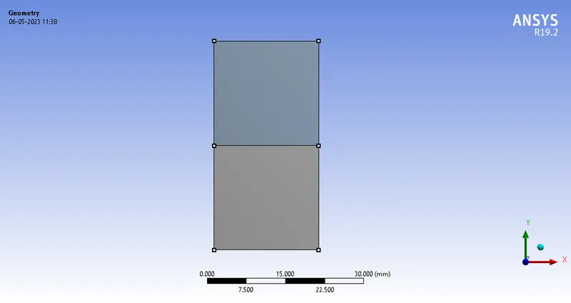
Two different rectangles one above the other is made to differentiate the two different fluids.

Dimensions of rectangle are : 20 X 20 m

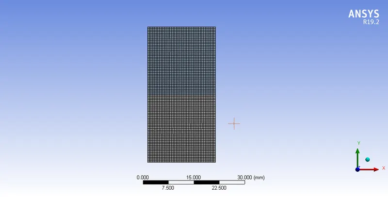
MESHING FOR CASE 1

MESH PARAMETERS
BASE MESH
Element size	0.5 mm
Max Element size	0.5 mm
Mesh Type	Quad
Nodes	3321
Elements	3200

SOLVER SETUP,

SOLVER INPUTS
Solver Time	Transient
Solver Type	Pressure Based
Gravity	- 9.81 in Y direction
Energy	Off
Models Method	Multiphase VOF
Materials	air & Water

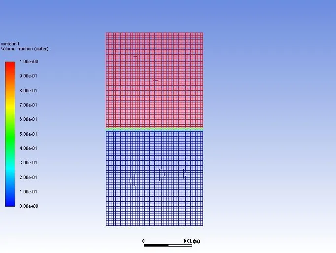
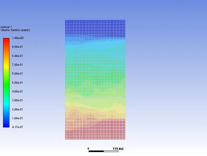
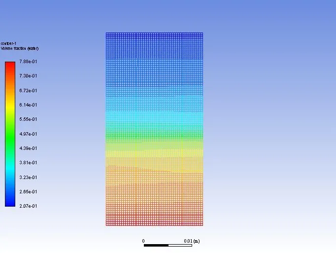
Volume Contour for case 1,

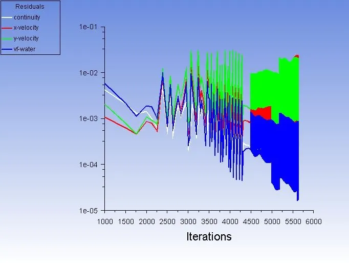
Residual Convergence plot for Case 1,

Instability phenomena for case 1 (air& water),

Animation File Link;

https://drive.google.com/file/d/1StSnIbY1eSOe5j7UwGuFhBR3D2gT55lJ/view?usp=share_link

MESHING

MESH PARAMETERS
BASE MESH 2
Element size	0.4 mm
Max Element size	0.4 mm
Mesh Type	Quad
Nodes	5151
Elements	5000

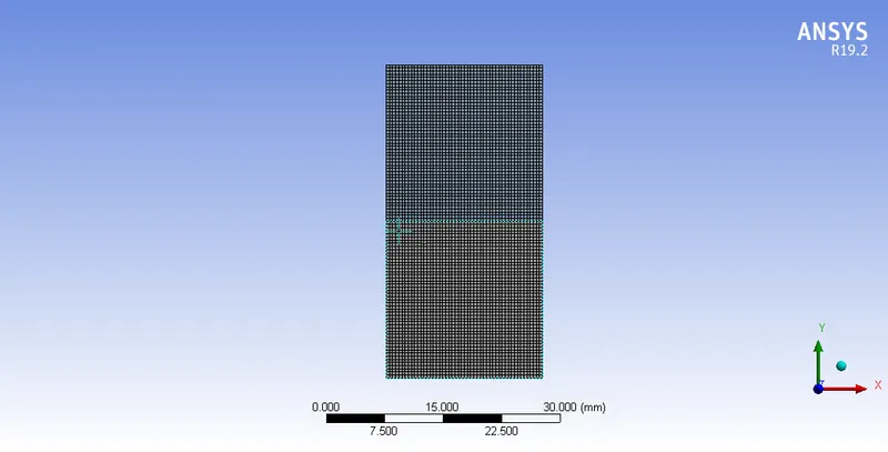
Volume Contour for case 1a,

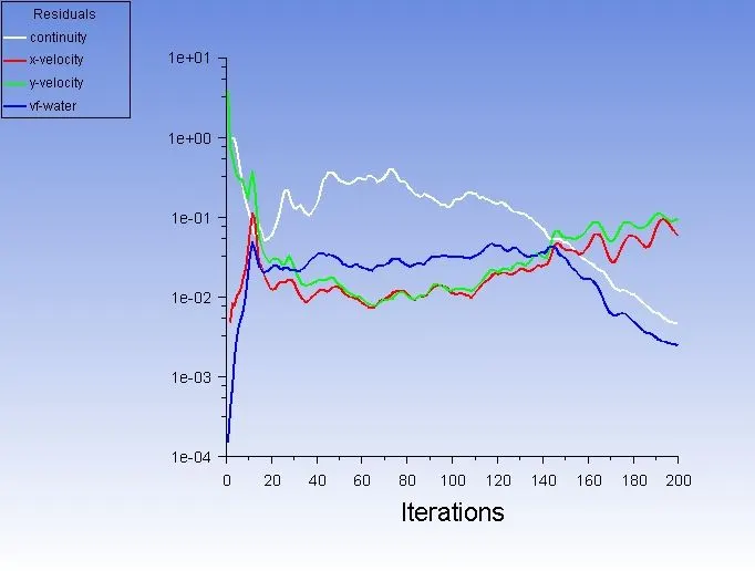
Residual Convergence plot for Case 1a,

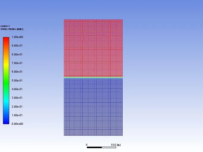
Instability phenomena for case 1a (air& water),

Animation File Link;

https://drive.google.com/file/d/14HwjanKjDNc5CzWVq9dQMngIjVxSd1jQ/view?usp=share_link

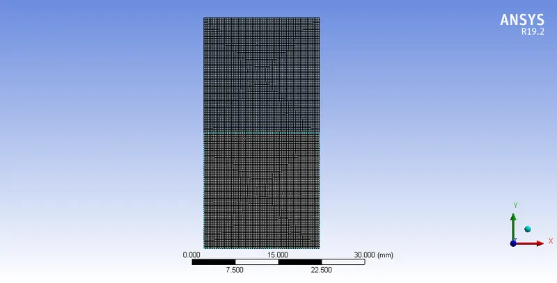
MESHING 2 FOR REFINED MESH (USER DEFINED MATERIAL AND WATER;

MESH PARAMETERS
Refined Mesh
Element size	0.3 mm
Max Element size	0.3 mm
Mesh Type	Quad
Nodes	9180
Elements	8978

SOLVER SETUP:

SOLVER INPUTS
Solver Time	Transient
Solver Type	Pressure Based
Gravity	- 9.81 in Y direction
Energy	Off
Models Method	Multiphase VOF
Materials	User defined Material(400 kg/m3 & 0.001 kg/ms) & Water

Volume Contour for Case 2,

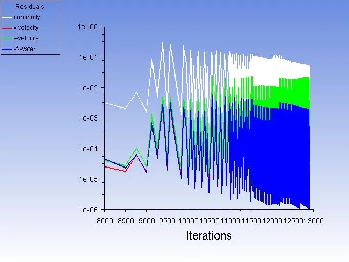
Residual Convergence plot for Case 2,

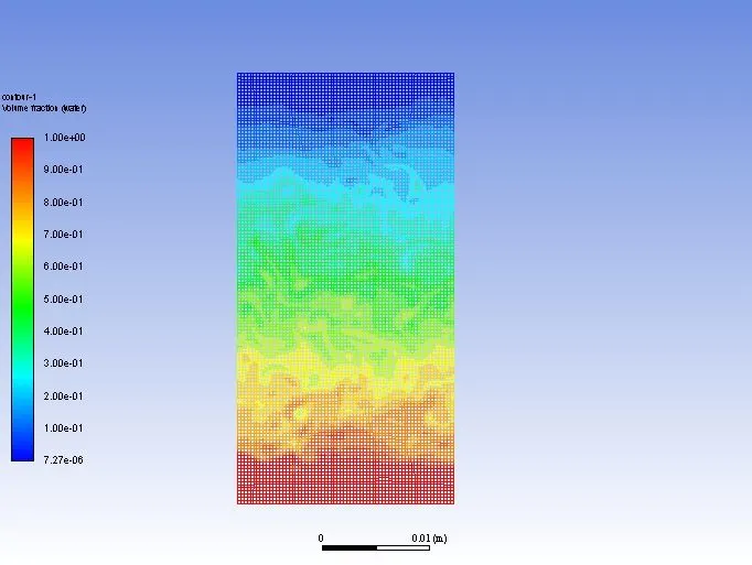
Instability phenomena for case 1 (user defined material & water),

Animation File Link;

https://drive.google.com/file/d/1aP3Fw4bXwUv4-qkMsP_TOZUW-vta7s5J/view?usp=share_link

Atwood number:

It is a dimensionless number in fluid dynamics used in the study of hydrodynamic instabilities in density stratified flows. It is a dimensionless density ratio defined as

A=(ρ1−ρ2)/(ρ1+ρ2)

where

ρ1= density of heavier fluid

ρ2= density of lighter fluid

Atwood number for the case 1; ,

A=(ρ1−ρ2)/(ρ1+ρ2)

where, ρ1= density of water, ρ2= density of air

A= (998.2-1.225)/(998.2+1.225)

A = 0.9975

Atwood number for case 2,

A=(ρ1−ρ2)/(ρ1+ρ2)

where, ρ1= density of water, ρ2 = density of user defined material

A = (998.2-400)/(998.2+400)

A = 0.4278

Significance of Atwood number to validate the variation of simulation result

• Significance:

• Penetration distance of the heavier fluid into the lighter fluid is given by the formula Agt^2 where g is the acceleration due to gravity and t is the time.

• For A close to 0, RT instability flows take the form of symmetric \"fingers\" of fluid.
• For A close to 1, the much lighter fluid \"below\" the heavier fluid takes the form of larger bubble-like plumes.
• When the Atwood number is so high the more instability takes place in the fluid and measuring the spikes of the instability is very difficult.
• When the Atwood number is low the more stable is the fluid mixture and measuring the spikes of the instability becomes possible because there exists a pattern of linear changes to certain limit.

Hence, the density and viscosity of the fluid plays an important role in defining the instability of the fluid and for Atwood number helps to distinguish the instability ranges.Therefore, the Rayleigh Taylor Instability for 2 different cases is carried out and the results are validated.