Week 5 - Rayleigh Taylor Instability

Rayleigh Taylor Instability

Aim: To study Rayleigh Taylor's Instability in Ansys Fluent

Objectives:

1. Study of some practical CFD models that have been based on the mathematical analysis of Rayleigh Taylor waves.
2. Perform the Rayleigh Taylor instability simulation for 2 different mesh sizes with the base mesh being 0.5 mm and compare results. select Air and Water for this simulation.
3. Run one more simulation with water and user-defined material (density = 400 kg/m³, viscosity = 0.001 kg/m-s) for refined mesh.
4. to define the Atwood Number. Find out the Atwood number for both cases and explain how the variation in the Atwood number in the above two cases affects the behavior of the instability.

Theory:

Rayleigh Taylor Instability

The Rayleigh-Taylor Instability (RTI) is seen when a heavy fluid is placed above a lighter fluid resulting in the instability of the interface into finger-like structures. When the fluids are confined by a small geometry, it is known that there is a critical depth in which the RTI can be suppressed.

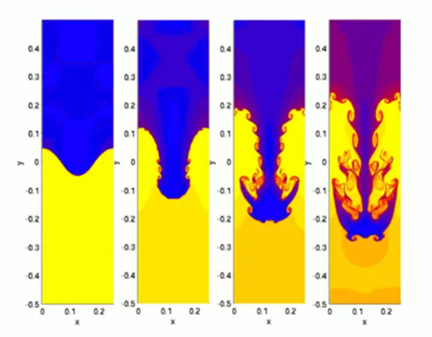
In CFD history, Practical CFD models that have been based on mathematical analysis for Rayleigh Taylor waves instability are

1. Kelvin-Helmholtz instability
2. Richtmyer-Meshkov instability
3. Plateau-Rayleigh instability

1. Kelvin-Helmholtz instability

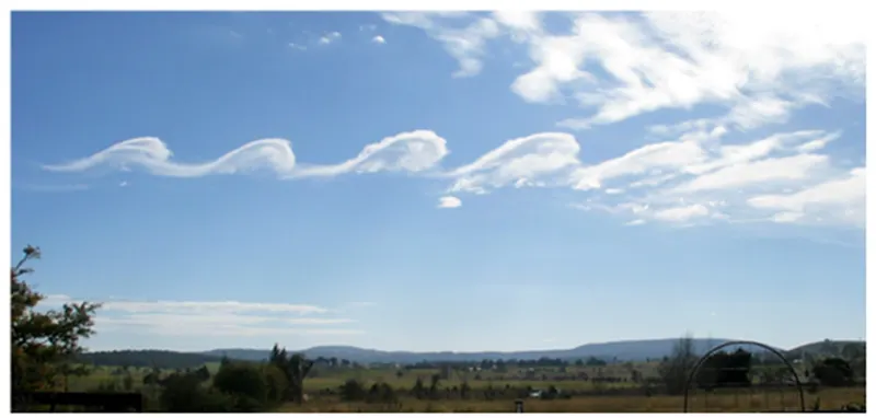
Kelvin–Helmholtz's instabilities were qualitatively described by Helmholtz and quantitatively analyzed by Kelvin. Instabilities of this kind frequently occur in nature, two such manifestations are the so-called “wind-over-water” and “clear air turbulence” instabilities. Consider two parallel streams of inviscid incompressible fluids superposed one above the other and assume that the upper and lower streams have positive and negative velocities, respectively. Since at the interface, there is a discontinuity in the velocity, the vorticity is a nonzero delta-function-like distribution which can be modeled as a vortex sheet. Consider a small sinusoidal perturbation of this sheet. For the two-dimensional flow in question, the vorticity is conserved under the motion of the fluid particles. Thus the vorticity has to induce a velocity in the positive (or negative) direction in parts of the sheet displaced upwards (or downwards). At the undisturbed points of the sine wave, the vorticity induces a rotational velocity which amplifies the wave and causes the instability to grow. As a result, the vorticity sheet develops vortex rolls and eventually breaks in a turbulent fashion. Kelvin–Helmholtz instability is global in nature and flow-specific. Since the basic mechanism is strongly affected by specific features of the underlying flow such as its shear, as well as physical forces such as gravity, viscosity, etc., it is very difficult, if not impossible, to describe Kelvin–Helmholtz's instabilities of generic flows.

In a frame of reference moving with the average velocity, the basic flow is symmetric and the wave therefore should have no preference between the positive and negative directions. The Kelvin–Helmholtz instability is caused by the destabilizing effect of friction, which overcomes the stabilizing effect of density stratification. The Kelvin–Helmholtz instability is commonly found in Earth’s atmosphere and ocean.

2. Richtmyer-Meshkov instability

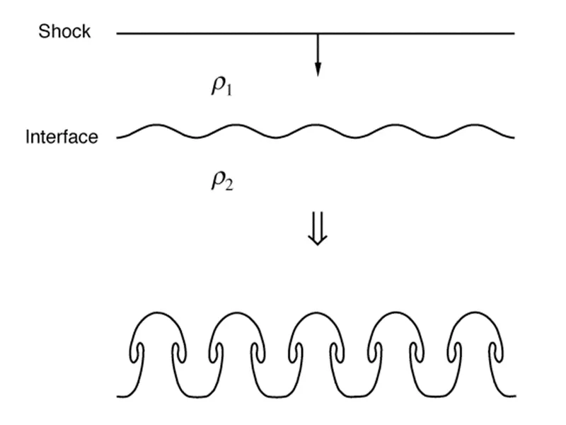
Richtmyer–Meshkov instability is the fluid flow phenomenon that occurs when a shock wave impinges (in the normal direction) upon an interface separating two gases having different densities. The instability causes perturbations on the interface to grow, producing vortical structures which potentially result in a turbulent mixing layer, as illustrated in the below figure.

The Richtmyer–Meshkov instability occurs in physical applications ranging from astrophysics to supersonic combustion. This instability is believed to occur when the outward propagating shock wave generated by the collapsing core of a dying star passes through the helium–hydrogen interface.

3. Plateau-Rayleigh instability

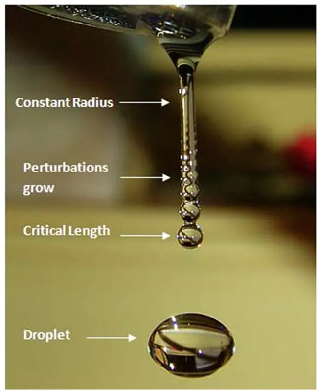
The Rayleigh-Plateau instability is defined by two factors: the growth rate of the perturbations and the length scale over which the instability grows. The time scale is equal to the length scale divided by the jet speed. The length scale is the length over which the fluid begins to decompose into droplets. The growth rate of the perturbations is important because it characterizes what disturbances initiate the instability. The disturbances are a set of sinusoids with varying growth rates and wavenumbers, only a limited number of which are unstable.

Solution & Results:

1. Preparation of gemoerty

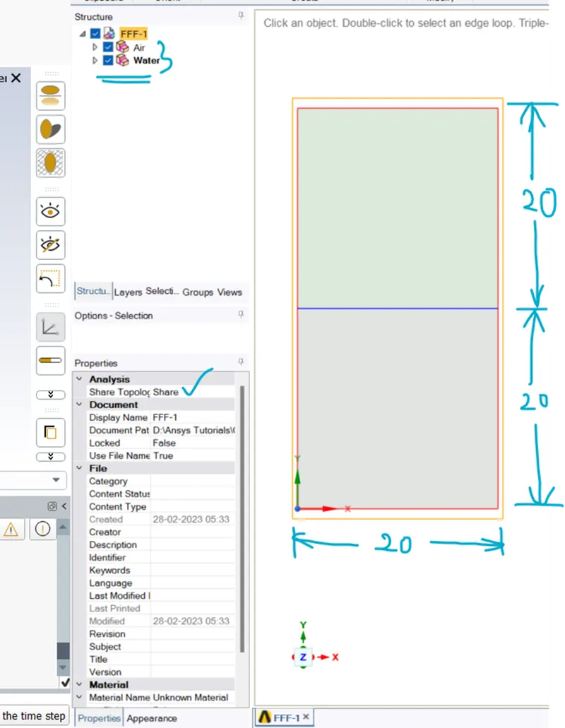
20 mm by 20 mm surface created using space claim for water and Air as shown below. Share topology is enabled.

2. Meshing

Case:1 - 0.5 mm mesh size with Air and Water

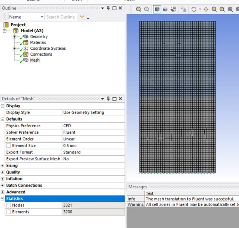
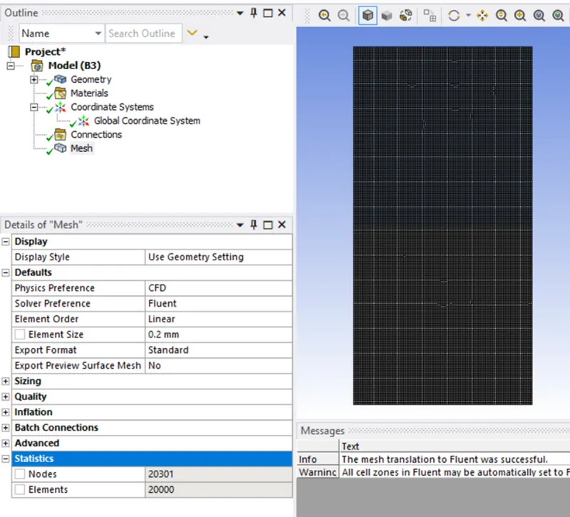
Case:2 - 0.2 mm mesh size with Air and Water & Case:3 - 0.2 mm mesh size with UDF (density = 400 kg/m³, viscosity = 0.001 kg/m-s) material and Water

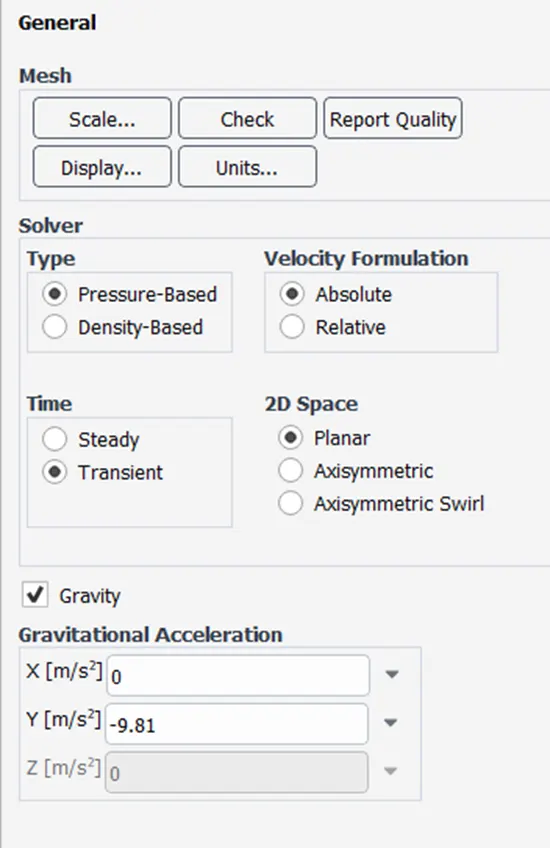
3. Fluent setup and solution

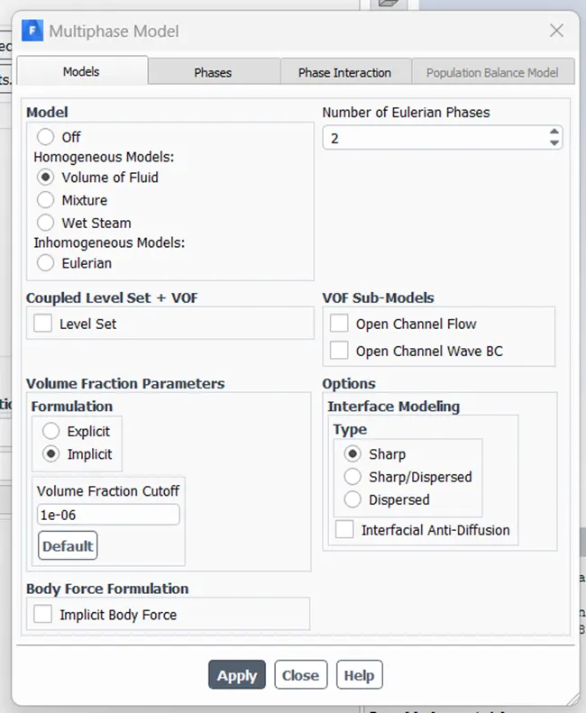
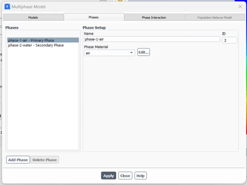
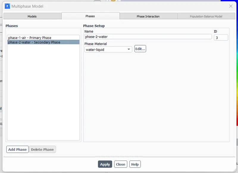
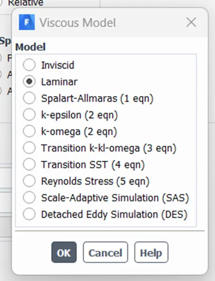
Initialization - Standard Initialization

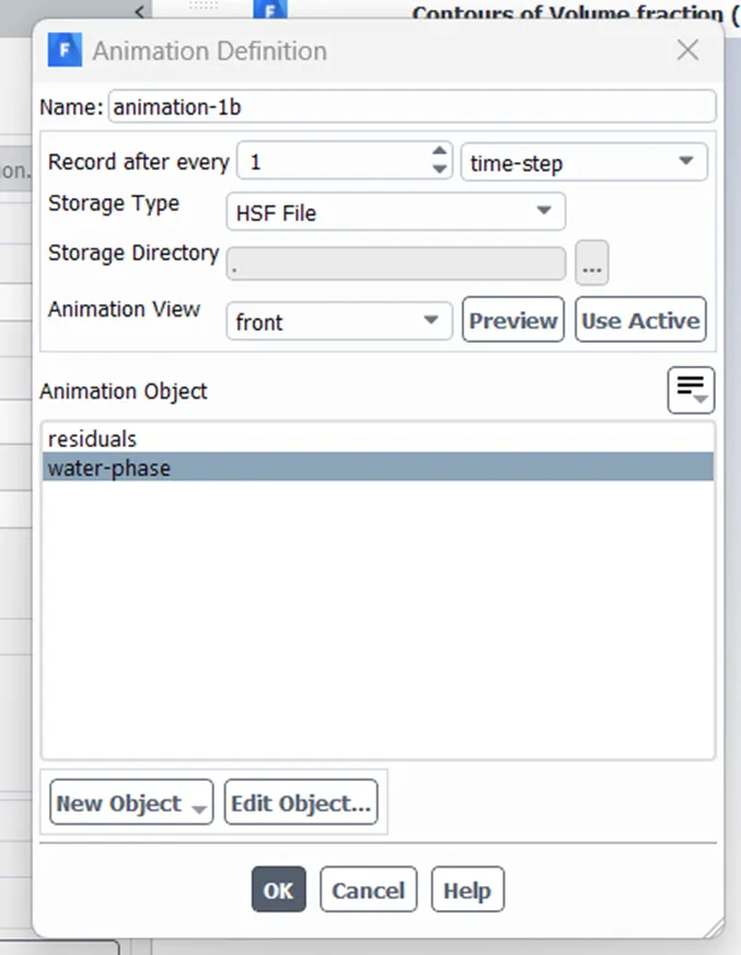
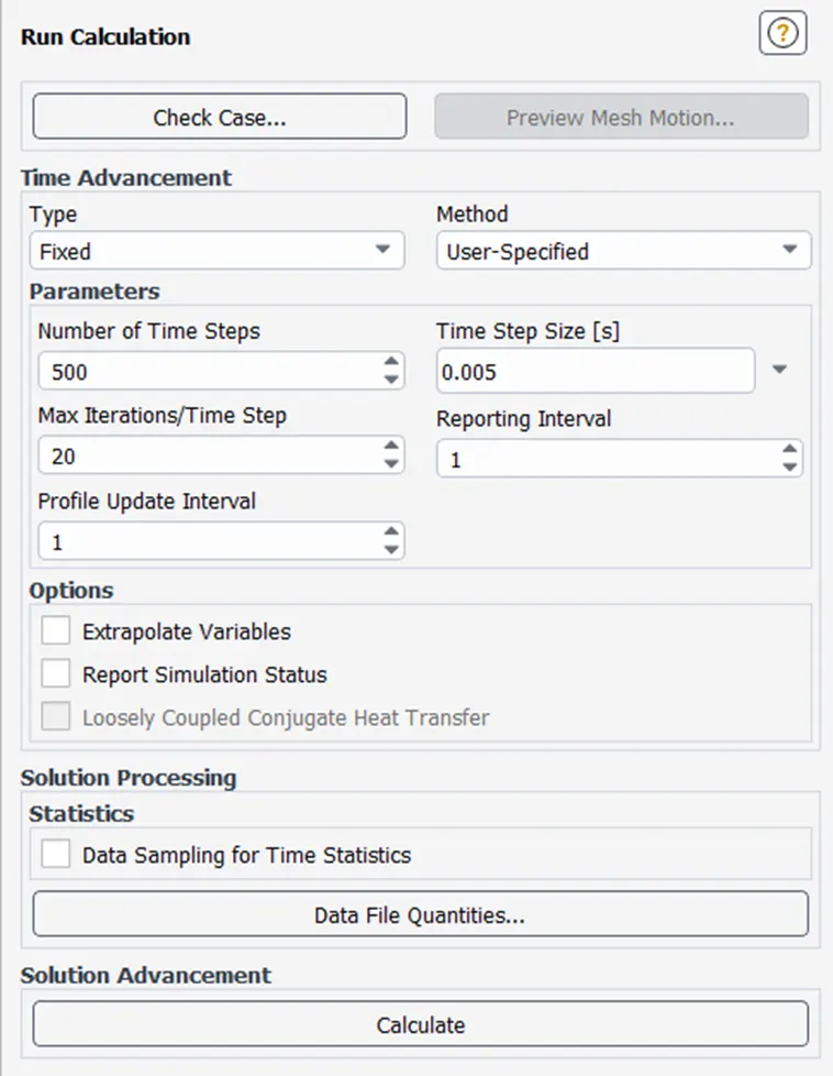
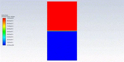
Create Animation - Water-Phase

4. Results

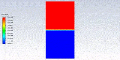
Case:1 - Animation

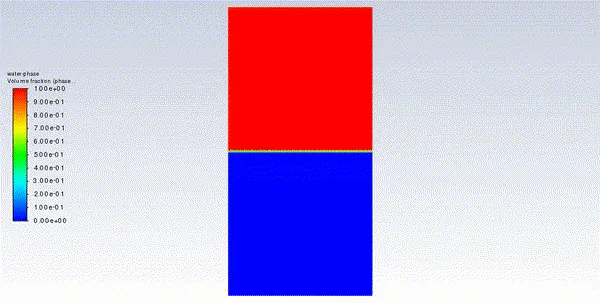
Case:2 - Animation

Case:3 - Animation (UDF)

Atwood Number:

The Atwood number is a dimensionless number in fluid dynamics used in the study of hydrodynamic instabilities in density-stratified flows.

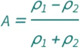
The Atwood number equals the ratio of the difference in mass densities to their sum.

FORMULA

symbol	description	physical quantity
A	Atwood number	"Atwood Number"
ρ1	the fluid density of the heavier fluid	"Mass Density"
ρ2	the fluid density of the lighter fluid	"Mass Density"

Variation in Atwood number:

the growth of bubble thickness is suppressed with the increase in stratification parameters(Sr) due to the density stratification at a small Atwood number (A_t) whereas it is enhanced at large A_t, because of the expansion and compression motions. The ratio of the bubble to spike thickness increases with the increase in Sr at any A_t. The effects of the flow compressibility on the molecular mixing fraction, Taylor Reynolds number, turbulent Mach number, and velocity divergence statistics are similar at different Atwood numbers.

Case 1 & 2: Atwood Number - 0.9975

Case 3: Atwood Number - 0.4278

Conclusion:

Rayleigh Taylor Instability simulation shows the interface of both fluids having different densities under the influence of gravity.

The following observations were made:

• Fine mesh generates the formation of bubbles and vortices beautifully. Computational time is more for fine mesh when compared with coarse mesh.
• Transient state analysis is preferred instead of steady state analysis to capture real-time data as the frequency of change is time-dependent.
• The Atwood number depends on the density of the fluid and ranges from 0 to 1.
• Both cases have larger Atwood numbers showing the Rayleigh Taylor Instability.

References:

1. http://www.scholarpedia.org/article/Richtmyer-Meshkov_instability_and_re-accelerated_inhomogeneous_flows
2. https://math.berkeley.edu/~mhegde/pdfs/Project%20Report%20-%20Fluid%20Mechanics%20and%20the%20Plateau-Rayleigh%20Instability.pdf
3. https://www.cambridge.org/core/journals/journal-of-fluid-mechanics/article/abs/effects-of-atwood-and-reynolds-numbers-on-the-evolution-of-buoyancydriven-homogeneous-variabledensity-turbulence/DC3ED87C2E774572B9D4E6FB0B688BB0
4. https://aip.scitation.org/doi/full/10.1063/5.0071437