Week 5 - Rayleigh Taylor Instability

Aim : To study and perform the Rayleigh Taylor instability simulation for different pair of fluids.

Objectives :

• Performing Multiphase simulation
• Introduction to VOF method
• Assigning material to the regions
• To perform mesh independent study
• Learn the patching of fluids in Ansys fluent

RAYLEIGH TAYLOR INSTABILITY

The Rayleigh–Taylor instability, or RT instability (after Lord Rayleigh and G. I. Taylor), is an instability of an interface between two fluids of different densities which occurs when the lighter fluid is pushing the heavier fluid. Examples include the behaviour of water suspended above oil in the gravity of Earth, mushroom clouds like those from volcanic eruptions and atmospheric nuclear explosions, supernova explosions in which expanding core gas is accelerated into denser shell gas, instabilities in plasma fusion reactors and inertial confinement fusion.

Water suspended atop oil is an everyday example of Rayleigh–Taylor instability, and it may be modeled by two completely plane-parallel layers of immiscible fluid, the denser fluid on top of the less dense one and both subject to the Earth's gravity. The equilibrium here is unstable to any perturbations or disturbances of the interface: if a parcel of heavier fluid is displaced downward with an equal volume of lighter fluid displaced upwards, the potential energy of the configuration is lower than the initial state. Thus the disturbance will grow and lead to a further release of potential energy, as the denser material moves down under the (effective) gravitational field, and the less dense material is further displaced upwards. This was the set-up as studied by Lord Rayleigh. The important insight by G. I. Taylor was his realisation that this situation is equivalent to the situation when the fluids are accelerated, with the less dense fluid accelerating into the denser fluid. This occurs deep underwater on the surface of an expanding bubble and in a nuclear explosion.

As the RT instability develops, the initial perturbations progress from a linear growth phase into a non-linear growth phase, eventually developing "plumes" flowing upwards (in the gravitational buoyancy sense) and "spikes" falling downwards. In the linear phase, the fluid movement can be closely approximated by linear equations, and the amplitude of perturbations is growing exponentially with time. In the non-linear phase, perturbation amplitude is too large for a linear approximation, and non-linear equations are required to describe fluid motions. In general, the density disparity between the fluids determines the structure of the subsequent non-linear RT instability flows (assuming other variables such as surface tension and viscosity are negligible here). The difference in the fluid densities divided by their sum is defined as the Atwood number, A. For A close to 0, RT instability flows take the form of symmetric "fingers" of fluid; for A close to 1, the much lighter fluid "below" the heavier fluid takes the form of larger bubble-like plumes.

Multiphase

Multiphase flow is a simulation(parallel) flow of materials with different states or phases(liquid-gas). It is a flow of materials with different chemical properties but in the same state or phase(liquid-liquid).

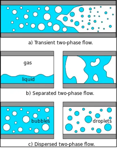
Types of Phases in Multiphase

1. Separated phase - It is defined as the one or more immiscible fluids in a continuous phase separated by an interface.
2. Mixed phase - It is defined as the phase in which one or more fluids are mixed together. It contains both separate and dispersed phases.
3. Dispersed phase - It is defined as the phase in which the finite number of phases are spread in the continuous phase.

Volume Of Fluid (VOF) Method

• Volume of fluid method is a surface tracking method.
• It is designed to find out the position of interface between the two or more immiscible fluids.
• The volume of fraction of each fluid in each of the cell through out domain can be tracked by using this method. Single set of momentum equations is shared only by the fluids.
• In this method all the control volumes must be filled with single phase or combination of phases.
• Application of the VOF model include stratified flows, free-surface flows, filling, sloshing, the motion of large bubbles in a liquid, the motion of liquid after a dam break, the prediction of jet breakup (surface tension) and the staedy or transient tracking of any liquid-gas interface.

COURANT NUMBER

The Courant–Friedrichs–Lewy or CFL condition expresses that the distance that any information travels during the time step length within the mesh must be lower than the distance between mesh elements. In other words, information from a given cell or mesh element must propagate only to its immediate neighbors.

The Courant number is a dimensionless value representing the time a particle stays in one cell of the mesh. It must be below 1 and should ideally be below 0.7. If the Courant number exceeds 1, the time step is too large to see the particle in one cell, it “skips” the cell. If it is smaller than 0.7, the particle stays in the cell for at least two time steps. The picture below visualizes this situation.

Example of a mesh comparing Courant number > 1 and Courant number <0.7

When the Courant number exceeds the value of 1, instabilities are amplified throughout the domain and may cause divergence of the simulation. Accordingly, to decrease the Courant number we can either:

• Decrease the time step Δt or
• Coarsen the mesh i.e. increase Δx

Best Practices

1. Make sure the sizes of the elements in the mesh do not differ too much. Measure the average cell size of your mesh. Let’s consider a case where it is about 1.7 mm.
2. Now have a look at your flow velocity, let’s assume it is 30 m/s. Accordingly, the average time a particle stays in one cell is 1.7e-3 / 30 = 5.67e-5 s.
3. This is the basis for defining the time step: To make sure your time is not too high set your initial time step to 10% this calculated value (in our case this would be 5.6e-6 s).
4. Multiply this time by the number of time steps you want to calculate to receive the value for the end time.

Enlisted below are some practical CFD models that have been based on the mathematical analysis of Rayleigh Taylor waves

• Kelvin-Helmholtz instability
• Richtmyer-Meshkov instability
• Plateau-Rayleigh instability

Kelvin–Helmholtz Instability

The Kelvin–Helmholtz instability (after Lord Kelvin and Hermann von Helmholtz) is a fluid instability that occurs when there is velocity shear in a single continuous fluid or a velocity difference across the interface between two fluids. Kelvin-Helmholtz instabilities are visible in the atmospheres of planets and moons, such as in cloud formations on Earth or the Red Spot on Jupiter, and the atmospheres of the Sun and other stars.

A KH instability rendered visible by clouds, known as fluctus, over Mount Duval in Australia

Kelvin-Helmholtz billows 500m deep in the Atlantic Ocean

Fluid dynamics predicts the onset of instability and transition to turbulent flow within fluids of different densities moving at different speeds. If surface tension is ignored, two fluids in parallel motion with different velocities and densities yield an interface that is unstable to short-wavelength perturbations for all speeds. However, surface tension is able to stabilize the short wavelength instability up to a threshold velocity.

If the density and velocity vary continuously in space (with the lighter layers uppermost, so that the fluid is RT-stable), the dynamics of the Kelvin-Helmholtz instability is described by the Taylor–Goldstein equation:

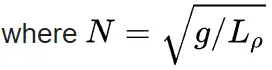
denotes the Brunt–Väisälä frequency, U is the horizontal parallel velocity, k is the wave number, c is the eigenvalue parameter of the problem, is complex amplitude of the stream function. Its onset is given by the Richardson number Ri. Typically the layer is unstable for Ri<0.25. These effects are common in cloud layers. The study of this instability is applicable in plasma physics, for example in inertial confinnnement fusion and the plasma-beryllium interface. In situations where there is a state of static stability, evident by heavier fluids found below than the lower fluid, the Rayleigh-Taylor instability can be ignored as the Kelvin–Helmholtz instability is sufficient given the conditions.

Numerically, the Kelvin–Helmholtz instability is simulated in a temporal or a spatial approach. In the temporal approach, the flow is considered in a periodic (cyclic) box "moving" at mean speed (absolute instability). In the spatial approach, simulations mimic a lab experiment with natural inlet and outlet conditions (convective instability).

Richtmyer–Meshkov Instability

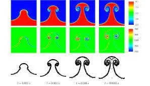
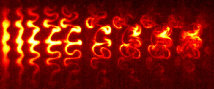
The Richtmyer–Meshkov instability (RMI) occurs when two fluids of different density are impulsively accelerated. Normally this is by the passage of a shock wave. The development of the instability begins with small amplitude perturbations which initially grow linearly with time. This is followed by a nonlinear regime with bubbles appearing in the case of a light fluid penetrating a heavy fluid, and with spikes appearing in the case of a heavy fluid penetrating a light fluid. A chaotic regime eventually is reached and the two fluids mix. This instability can be considered the impulsive-acceleration limit of the Rayleigh–Taylor instability.

Plateau-Rayleigh Instability

The Plateau–Rayleigh instability, often just called the Rayleigh instability, explains why and how a falling stream of fluid breaks up into smaller packets with the same volume but less surface area. It is related to the Rayleigh–Taylor instability and is part of a greater branch of fluid dynamics concerned with fluid thread breakup. This fluid instability is exploited in the design of a particular type of ink jet technology whereby a jet of liquid is perturbed into a steady stream of droplets.

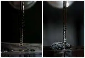
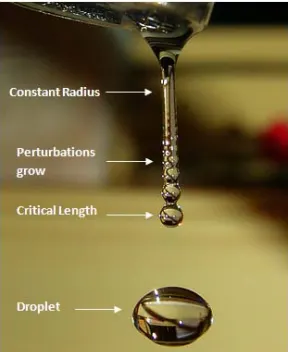
The driving force of the Plateau–Rayleigh instability is that liquids, by virtue of their surface tensions, tend to minimize their surface area. A considerable amount of work has been done recently on the final pinching profile by attacking it with self-similar solutions.

STEPS USED FOR SIMULATIONS

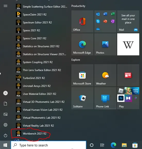
Click on red encircled "Workbench 2021 R2" as shown in the above image to start the simulation.

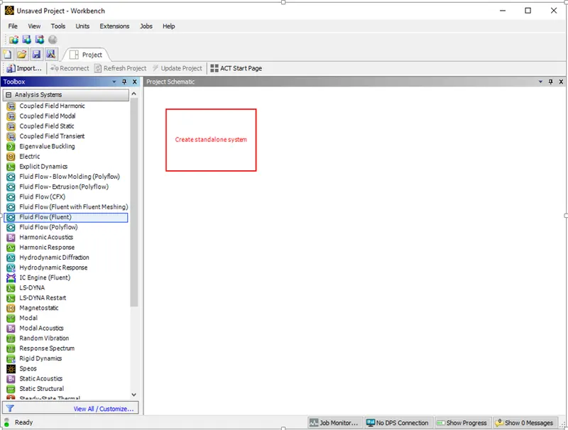
Click On Fluid Flow (Fluent) under Analysis Systems and drag it to create a standalone system.

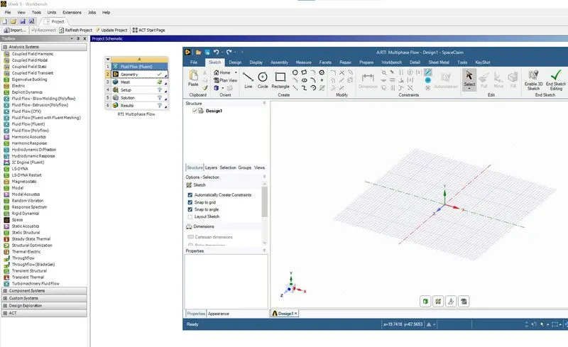
Rename the Project by using the left click and then click the Geometry.

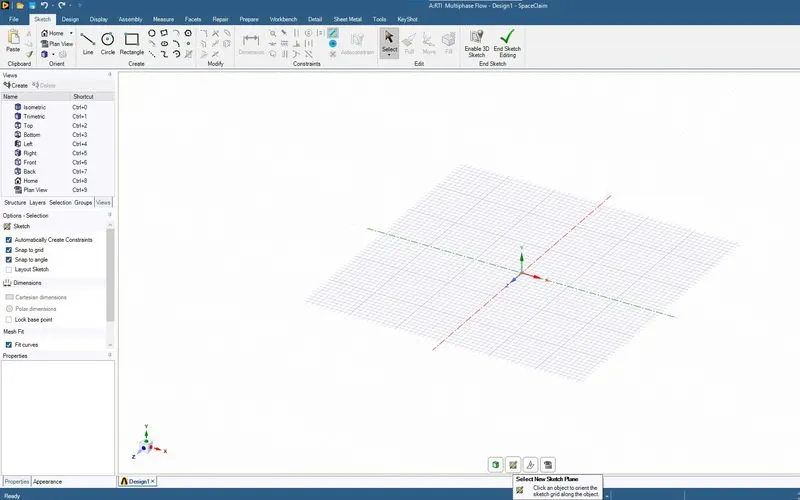
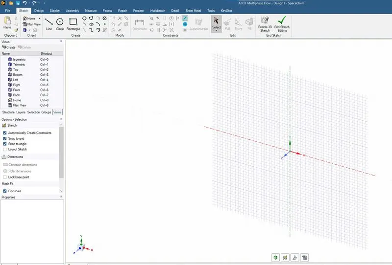
Using the sketch plane we select the XY plane as shown in the above two images.

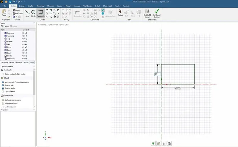
Using the Rectangle under sketch we draw a rectangle as shown in the above image.

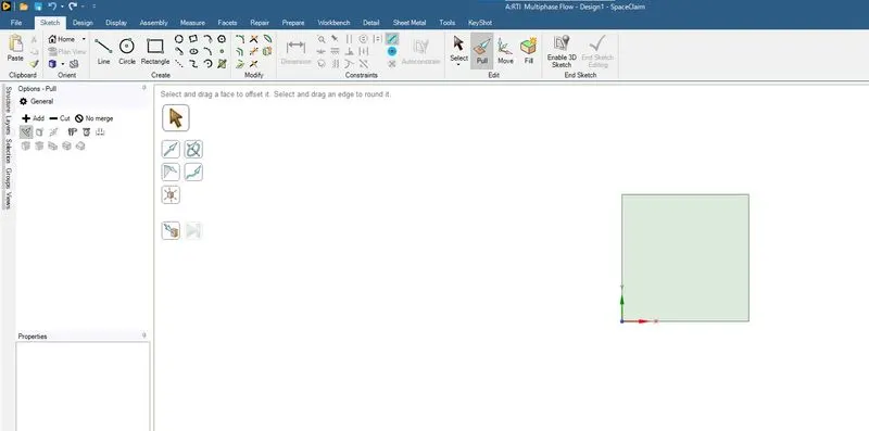
Using the pull command a sketch is converted into surface.

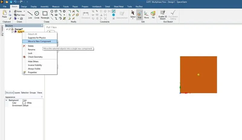
The surface is moved to a new component which is named as Air using the method as shown in the above image.

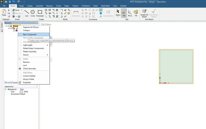
A new component water is made as shown in the above image.

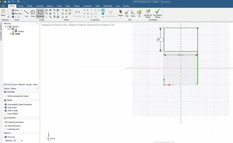
Using the rectangle under the sketch a square of 20mm x 20mm is made above the air as shown in the above image.

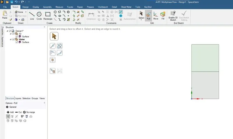
Using the pull command as shown in the above image the sketch for water is converted to surface.

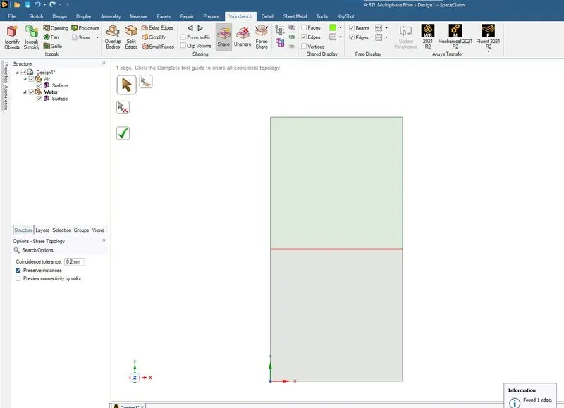
Using the share topology the common is shared between the air and water for meshing.

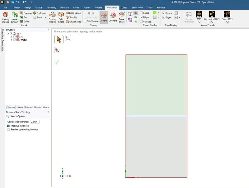
Thespacalaim is closed and the next step is meshing.

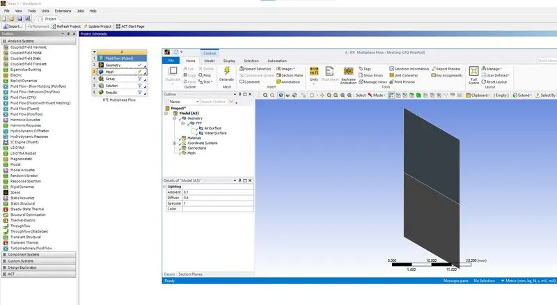
Meshing module is started as shown in the above image. THe appearance of window as shown in the above image.

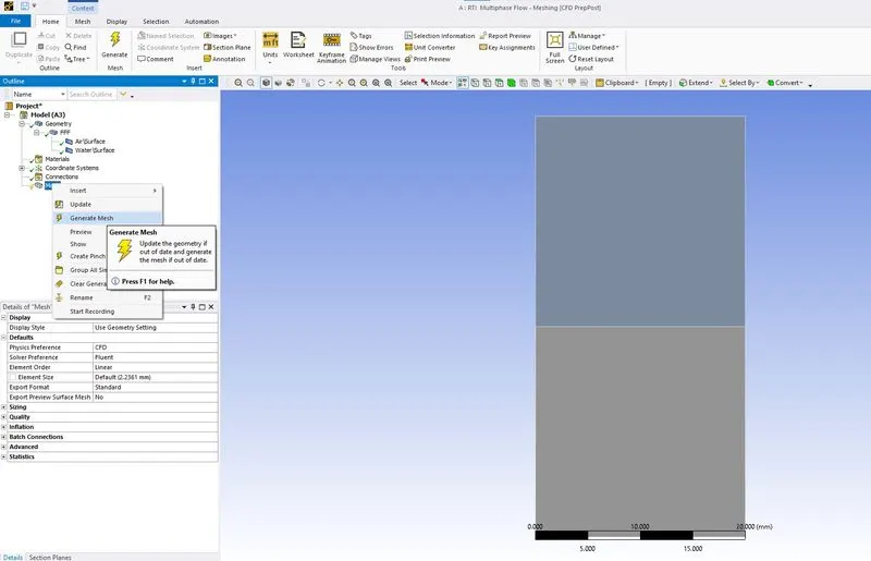
Using the Generate Mesh as shown in the above image, the default mesh is generated.

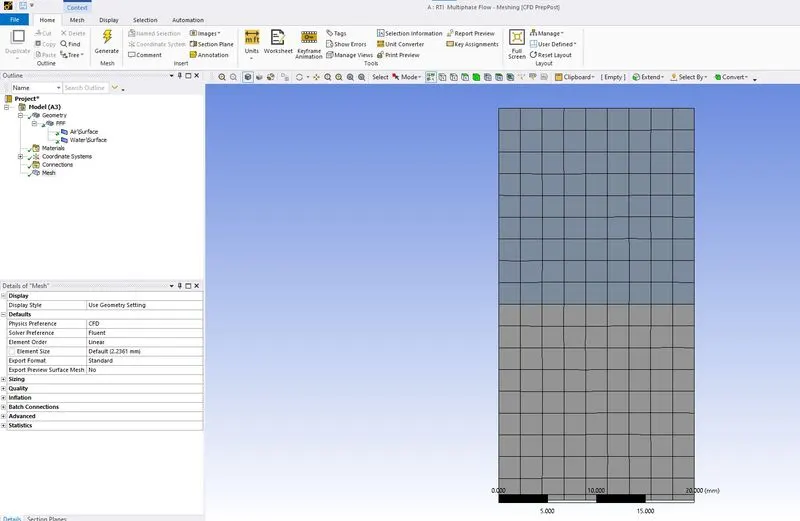
THe default mesh generated is as shown in the above image.

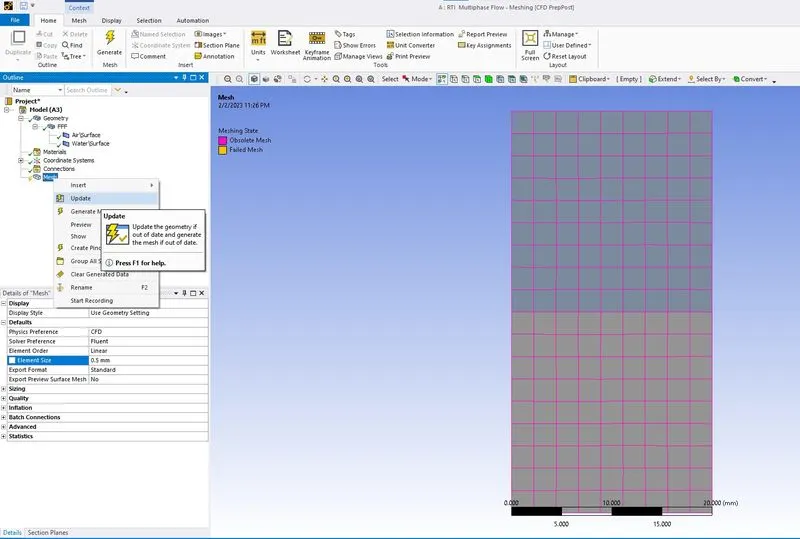
THe mesh is refine by changing the element size to 0.5mm and update is donw as shown in the above image.

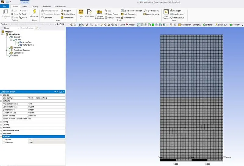
The refined mesh with element size of 0.5mm.

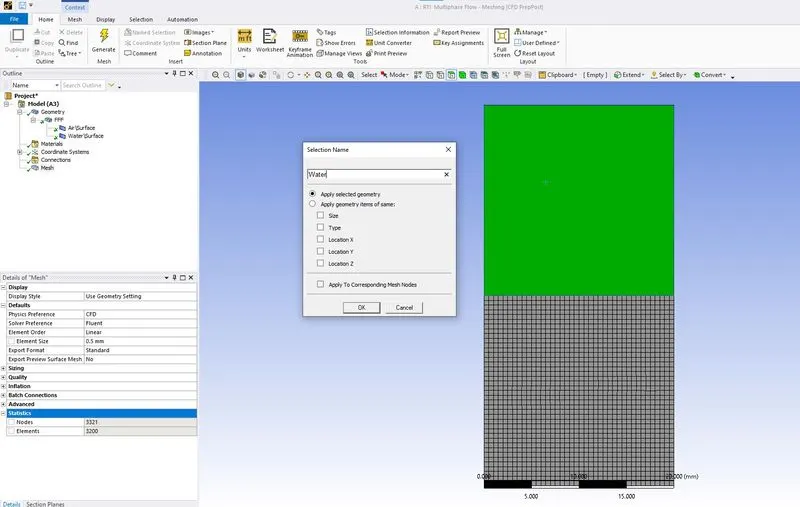
Using the named selection the selected surface is named as Water.

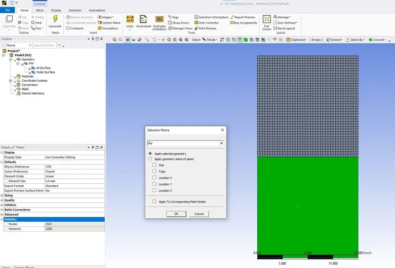
Using the named selection the selected surface is named as Air. The meshing module is closed now.

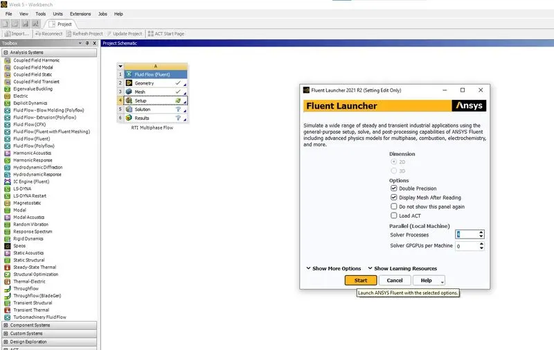
THe fluent set up is started as shown in the above image.

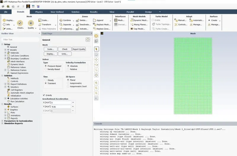
Under the general set up in time, transient is selected, gravity is enabled as shown in the above image.

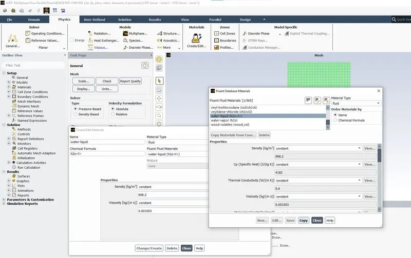
Using the fluid fluent material database a material named water is added to the default air.

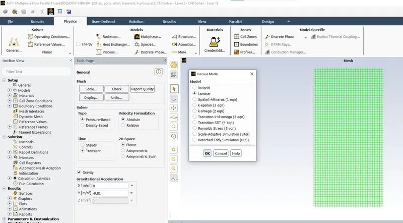
Under the Models in viscous the Laminar is selected as the viscous model as shown in the above image.

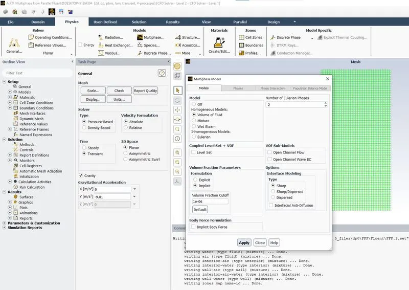
Under the Multiphase Model, Volume Of Fluid (VOF) is selected under Homogenous models and Volume Fractions Parameters is changed to Implicit as shown in the above image.

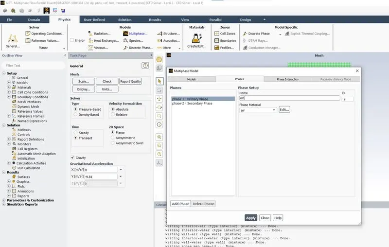
In the phases under multiphase model phase-1 is change to air as shown in the above image.

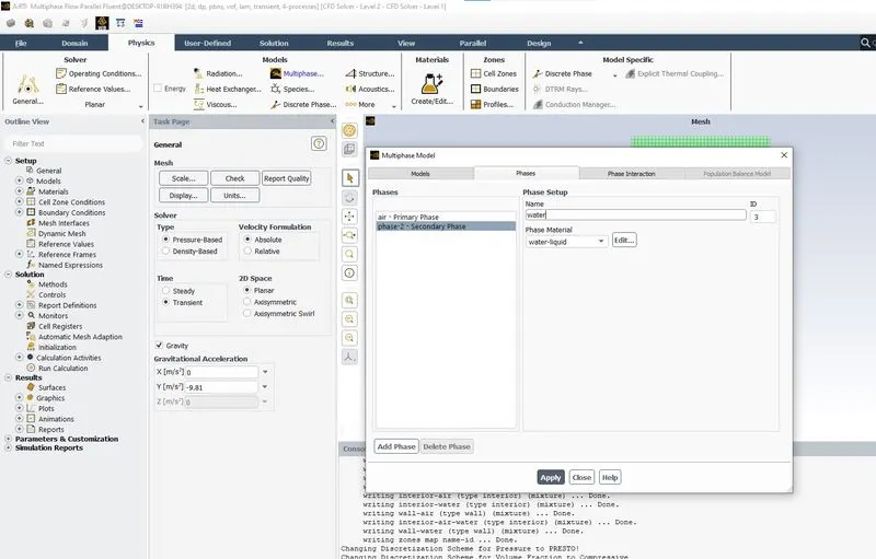
In the phases under multiphase model phase-2 is changed to water as shown in the above image.

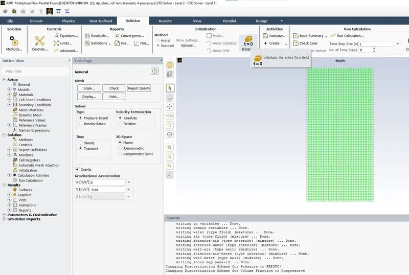
Initialization is done as shown in the above image.

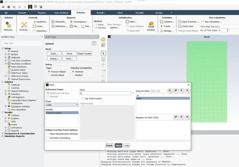
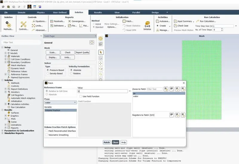
After initialization, patching is done as shown in the above two images.

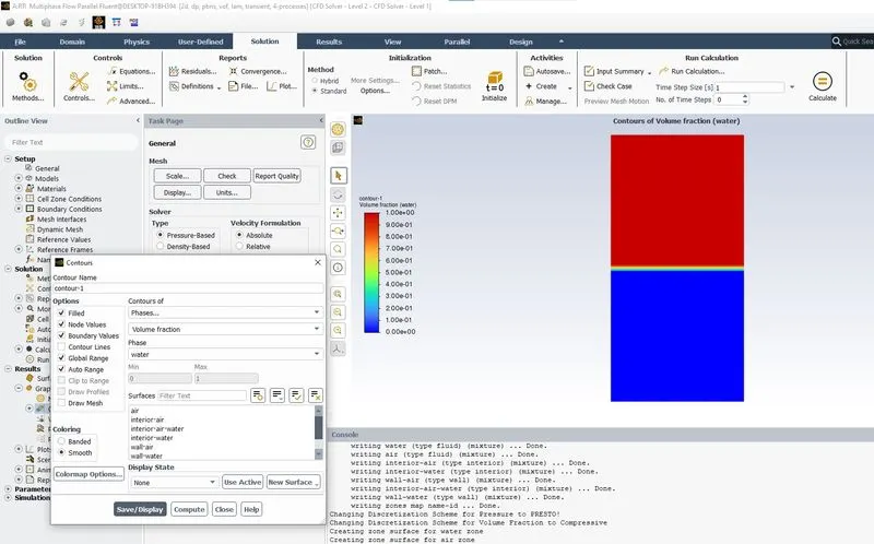
A contour of Volume fraction is defined as shown in the above image.

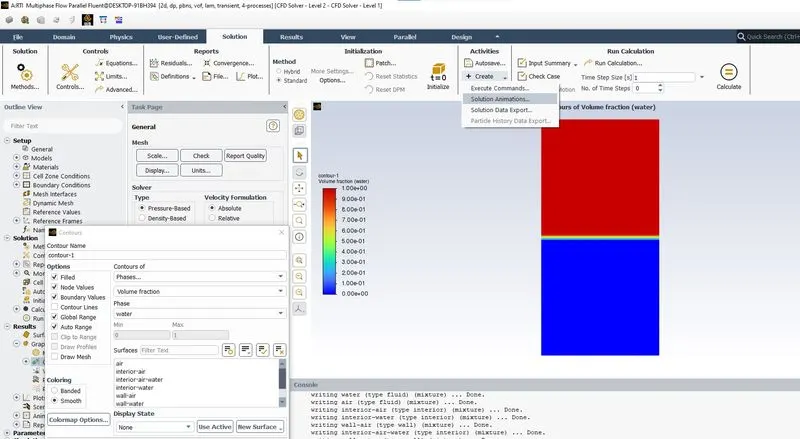
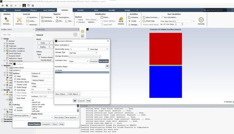
The solution animation is set as shown in the above two images.

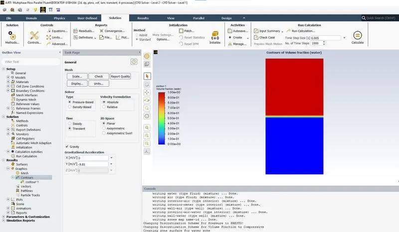
A calculation is run for the time step size of 0.005s & number of time steps as 1000 as shown in the above image.

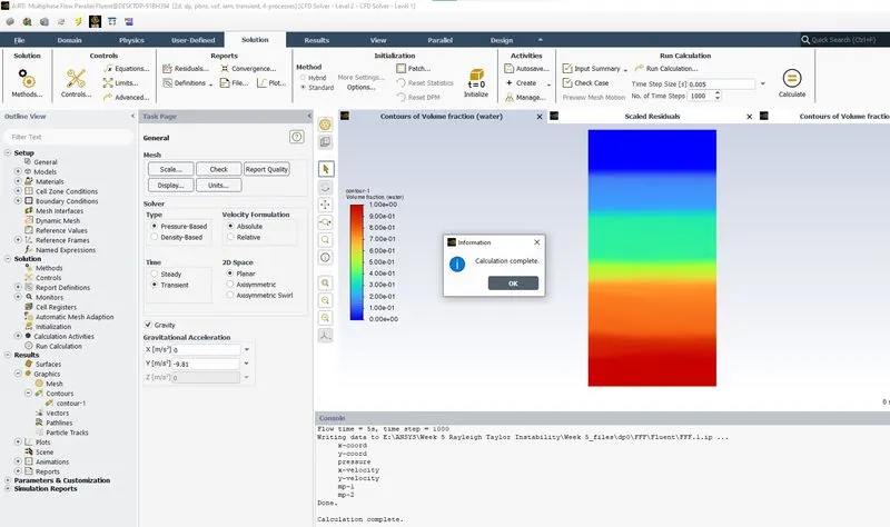
The final contour image after the calculation is complete.

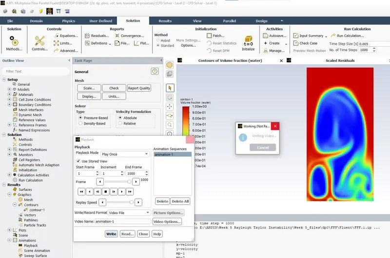
The method to write the animation to desired video file for us to playback.

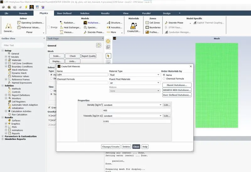
The method to define the user defined material as shown in the above image.

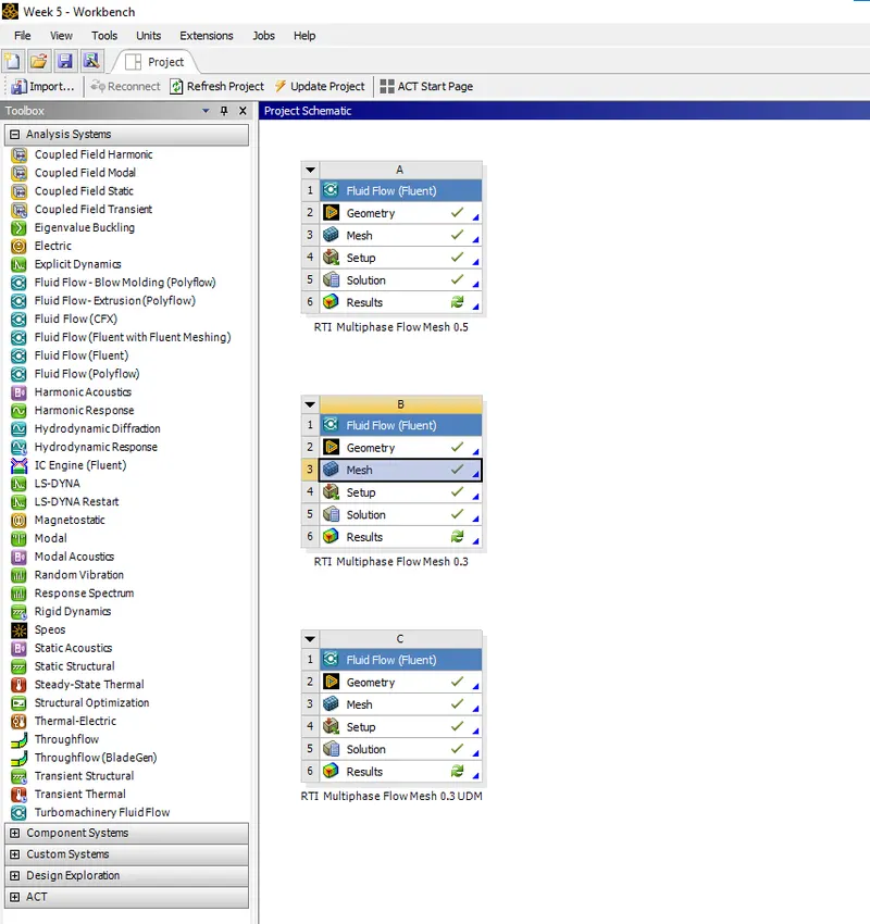
Case 1 : Mesh of 0.5mm element size (Air & Water)

1.1 Animation Video

https://drive.google.com/file/d/1rC-TQ94Y8QhWG8zvNla2SxCdpdw9nH7v/view?usp=sharing

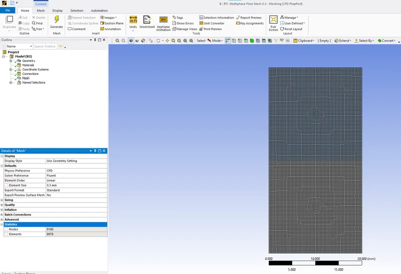
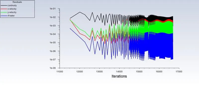
Case 2 : Refined Mesh of 0.3mm element size (Air & Water)

2.1 Mesh Elements

2.2 Scaled Residuals

2.3 Contours of Volume Fraction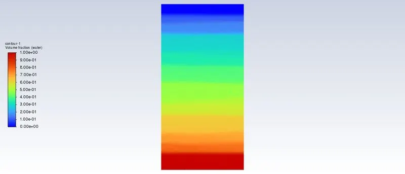

2.4 Animation Video

https://drive.google.com/file/d/1TFnHDGxao6L6jD4lE3_V7jvVxBTYQjzB/view?usp=sharing

Case 3 : Refined Mesh of 0.3mm element size (UDM & Water)

3.1 Mesh Elements

3.2 Scaled Residuals

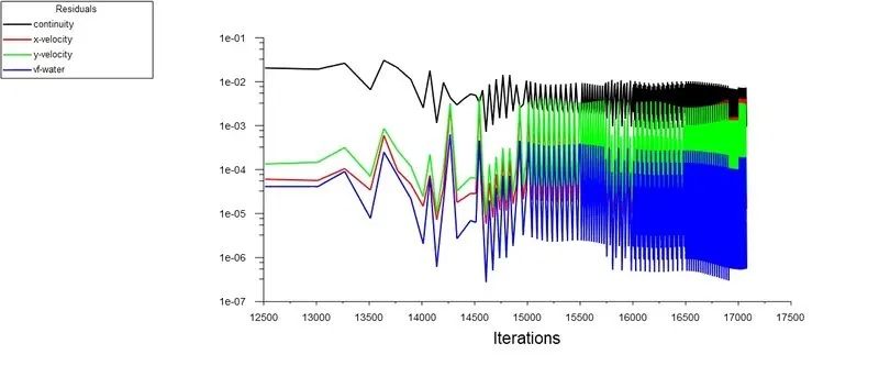
3.3 Contours of Volume Fraction

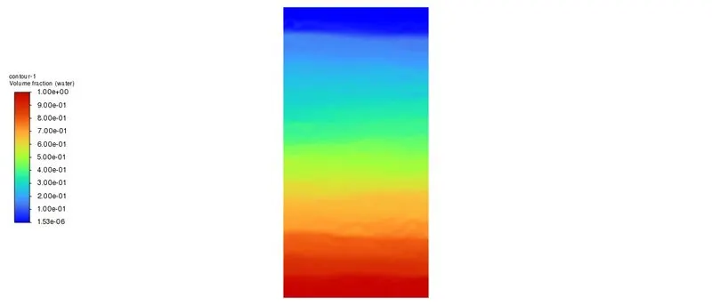
3.4 Animation Video

https://drive.google.com/file/d/1Rdp4KuzdstDkYHE1HeTsSt8gR4c9z8H1/view?usp=sharing

ATWOOD NUMBER

The Atwood number (A) is a dimensionless number in fluid dynamics used in the study of hydrodynamic instabilities in density stratified flows. It is a dimensionless density ratio defined as

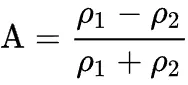
where

ρ1 = density of heavier fluid

ρ2 = density of lighter fluid

Case 1 & 2

ρ1 = density of heavier fluid = 998.2 Kg /m^3

ρ2 = density of lighter fluid = 1.225 Kg / m^3

A = (998.2-1.225) / (998.2+1.225) = 996.975 / 999.425 = 0.9975

Case 3

ρ1 = density of heavier fluid = 998.2 Kg /m^3

ρ2 = density of lighter fluid = 400 Kg / m^3

A = (998.2-400) / (998.2+400) = 598.2 / 1398.2 = 0.4278

CONCLUSION

• Finer Mesh captures the instability better than the coarse mesh but it takes more time for the heavier fluid to settle down.
• When the Atwood number is close to 1, the much lighter fluid below the heavier fluid takes the form of larger bubbles like plumes.
• For Atwood numbers close to 0, RT instability flows take the form of symmetric figures of fluid.
• Therefore, from the value of the Atwood number, it is seen from the simulations that air forms larger bubbles when water is poured down the air pushes through and forms large bubbles. Therefore, the results can be validated by obtaining the value of the Atwood number. Atwood number is an important parameter in the body of Rayleigh Taylor's instability.