Week 5 - Rayleigh Taylor Instability
AIM:
- What are some practical CFD models that have been based on the mathematical analysis of Rayleigh Taylor waves? In your own words, explain how these mathematical models have been adapted for CFD calculations.
- Perform the Rayleigh Taylor instability simulation for 2 different mesh sizes with the base mesh being 0.5 mm. Compare the results by showing the animations( Attach them from your google drive). Observe the differences in the animation and explain the effect of mesh size on simulation. Also, explain why a steady-state approach might not be suitable for these types of simulation.[ Choose Air and Water for this simulation]
- Run one more simulation with water and user-defined material(density = 400 kg/m3, viscosity = 0.001 kg/m-s) for refined mesh.
- Define the Atwood Number. Find out the Atwood number for both the cases and explain how the variation in Atwood number in the above two cases affects the behavior of the instability.
Rayleigh Taylor Instability:
The Rayleigh-Taylor instability is a fluid dynamic instability that occurs when a fluid of lower density is placed above a fluid of higher density in a gravitational field. The instability is characterized by the growth of small perturbations in the density interface between the two fluids, leading to the formation of "fingers" or "mushrooms" of the denser fluid that penetrate the lighter fluid. This instability is commonly observed in astrophysics, but can also be found in other scientific disciplines such as geophysics, oceanography and combustion science. The instability is named after Lord Rayleigh and G.I. Taylor, who independently described it in the late 19th and early 20th centuries.
Practical CFD models
There are several practical CFD (computational fluid dynamics) models that have been developed based on the mathematical analysis of Rayleigh-Taylor instability. Some examples include:
-
The level set method: This is a widely used method for simulating the dynamics of fluid interfaces. The level set method tracks the position of the fluid interface by representing it as the zero level set of a scalar function, called the level set function.
-
The volume-of-fluid (VOF) method: This is another popular method for simulating fluid interfaces. The VOF method represents the fluid interface as a discontinuity in the fluid density.
-
The front-tracking method: This method is particularly well-suited for simulating the dynamics of sharp fluid interfaces, such as those that occur in Rayleigh-Taylor instability. The front-tracking method tracks the position of the fluid interface by following the motion of a set of discrete points that lie on the interface.
-
The marker-and-cell method: This is a hybrid method that combines the VOF and front-tracking methods. The marker-and-cell method uses a set of discrete markers to track the motion of the fluid interface, while the fluid properties are represented using a finite volume method.
These are some of the methods that have been applied to model RT instability, but depending on the specific problem, other methods like Lattice Boltzmann method and Finite difference method can also be used.
Atwood number
The Atwood number (A) is a dimensionless number in fluid dynamics used in the study of hydrodynamic instabilities in density stratified flows. It is a dimensionless density ratio defined as

where
ρ1= density of heavier fluid
ρ2= density of lighter fluid
SOLVING & MODELLING APPROACH
- Construct a 2D geometry for the 2 fluid phases.
- Mesh independence study is carried out for different mesh length.
- Laminar Transient state with volume of fluid mode is used
- The simulation is calculated for very small time steps to avoid floating point error.
- Animations are created to analyse the flow patterns
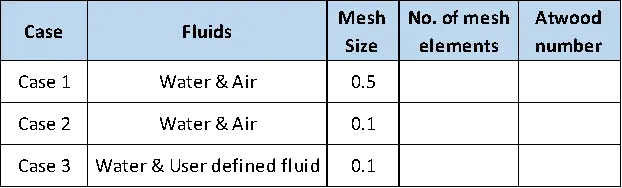
Total Cases.
PRE PROCESSING AND SOLVER SETTING
In our challenge we will create a flow simulation of Rayleigh Taylor Instability. In general I will be explaining only one case and posting the screenshots of the other cases.
Case 1
Mesh size - 0.5mm,
Fluid - Water and air
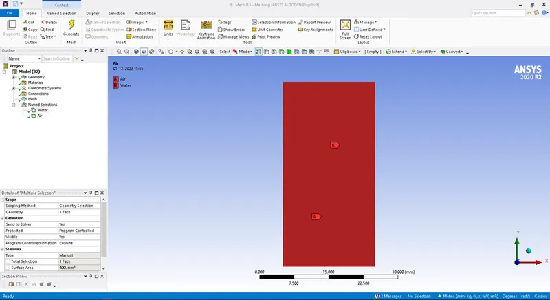
Step 1 : Open the geometry Space Claim. Two square with 20x20mm is drawn one over the other for the two fluids. Once this is done the topology is shared so the meshing will be smooth.
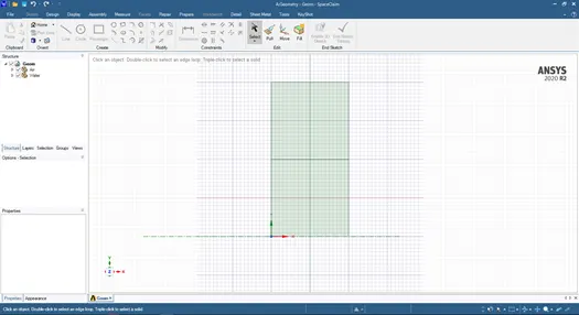
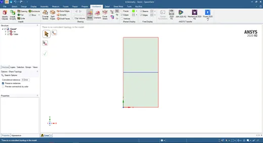
Once this process is done. We will close the space claim and open the mesh module.
Step 2 : Open the mesh module and under the mesh details give CFD Fluent as preference and Element size of 0.5mm. But since we are going to go for mesh independence study uniform meshing size is maintained throughout the volume. Note the number of nodes and elements for the study.
After the meshing is done check for the quality criterion. Check whether the mesh quality is above 5%. Once this is done name the faces of the volume as Water and air.
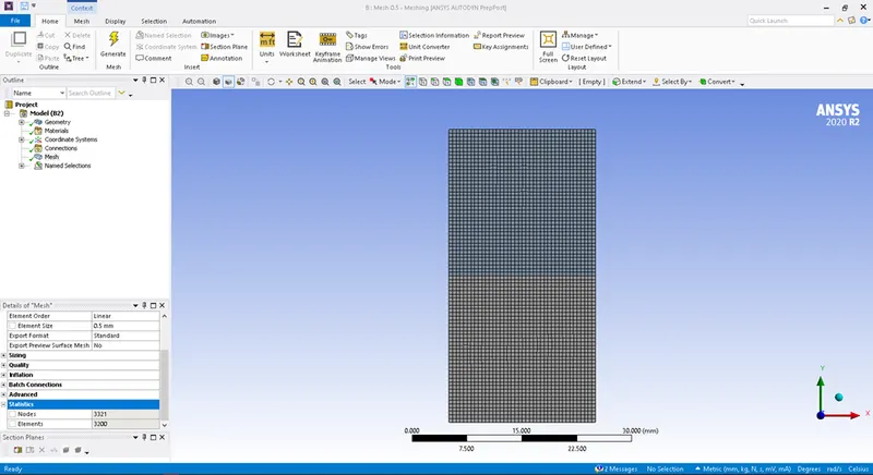
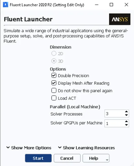
Step 3 : After the meshing and face naming are done move on to Fluent Solver. In the fluent launcher select double precision, display mesh after reading and give the appropriate solver processors and GPUs.
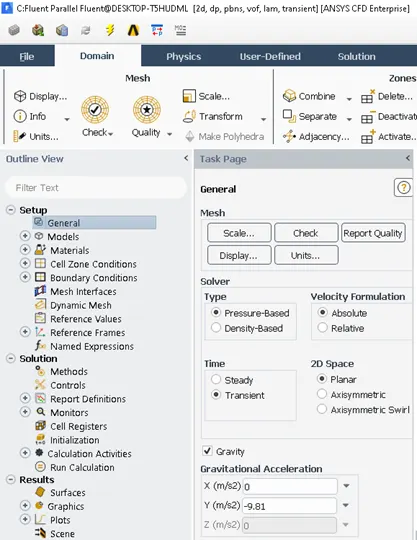
In the ANSYS CFD we need to give all the conditions, parameters and models. To start with go to physics menu and click general settings. In that select Pressure based type solver, Absolute velocity formulation and transient state flow. Next we need to give the model. For this case Laminar is selected.
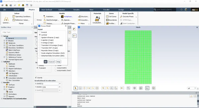
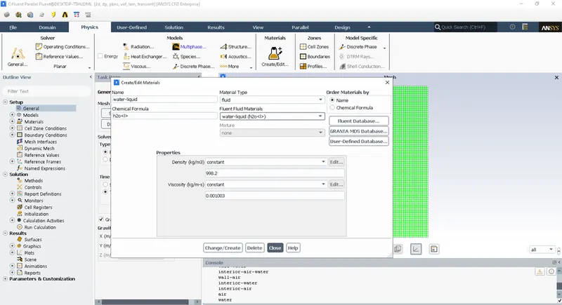
Next is the flow material selection. By default air is selected. We have two fluid phases. Hence select water from the fluent database.
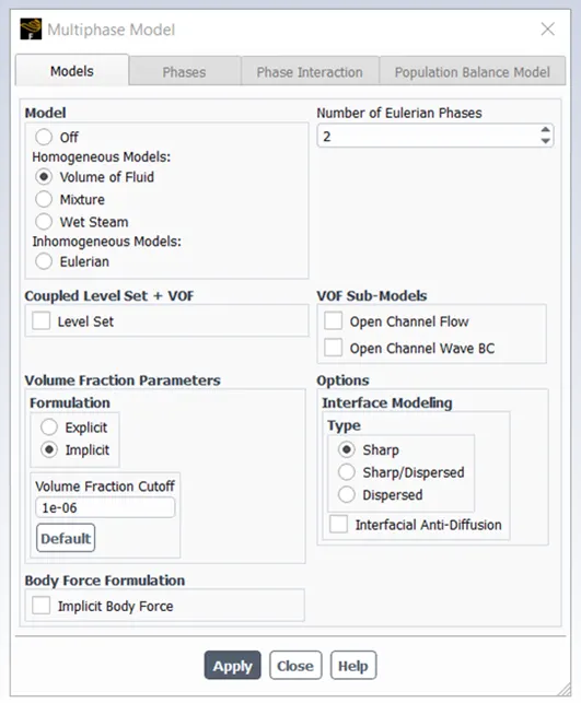
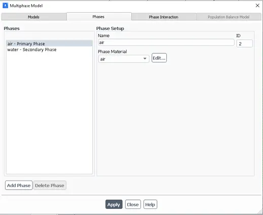
Click on the multiphase and select volume of fluids with two fluids. In the phases tab rename and assign the primary and secondary phases.
After the physics part is done move to the solution part. Initialise the simulation first. click Initialize to initialize the boundary conditions. Hybrid method is selected before initialization. Click on Autosave to obtain a animation of the flow in the post results.

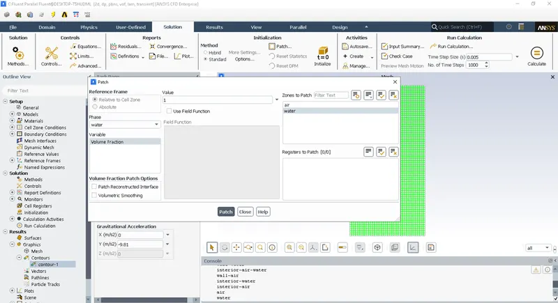
Patch the created region with the lubricating fluid. Set the fluid and select volume fraction. Set the values to 1 and 0.
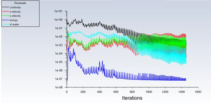
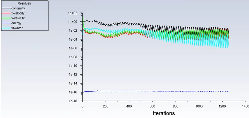
Then run the calculation for a given number of iterations till the convergence is obtained. Depending upon the number of elements and model selected the time required for convergence varies. In the CFD module itself we can compute, measure, plot, animate, etc., if needed.
Step 4 : After the solutions and calculations move to the result module to get different graphs, plots, contours, animations etc.,. Sectional views can be created if required.
RESULTS
Case 1
Mesh size - 0.5mm,
Fluid - Water and air
Residual Plot:
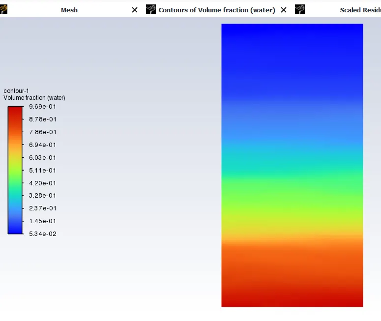
Contours of volume fraction:
Animation Video: https://drive.google.com/file/d/1j3cq_dRcv7mLpg5RcEkb5OkJcckRXBYy/view?usp=sharing
Mesh size - 0.1mm,
Fluid - Water and air
Residual Plot:
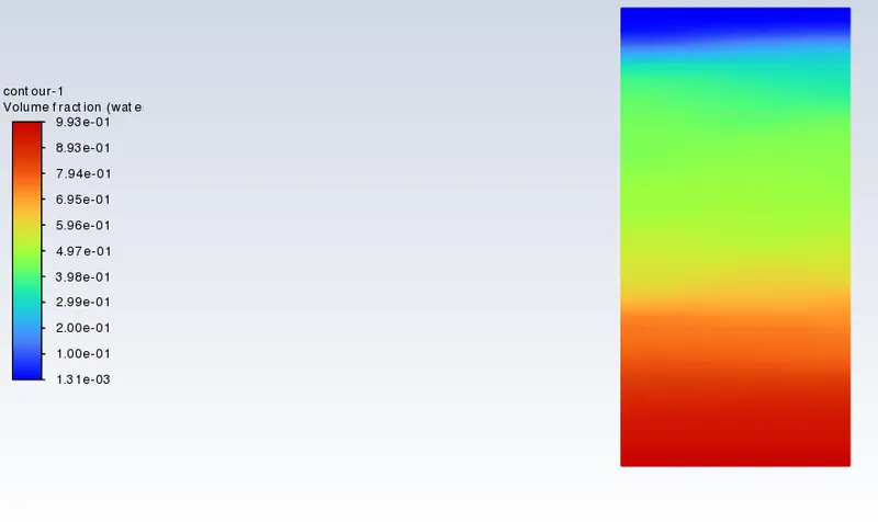
Contours of volume fraction:
Animation Video: https://drive.google.com/file/d/1cNBwedz2cK42GBrkb01j6oUGnvqUmR9X/view?usp=sharing
Case 3: refined mesh with an elemental size of 0.3mm and having the user material and water.
elements=3200
timestep size=0.025
no. of timestep=170
Mesh
Atwood Number
It is a dimensionless number that is used to study hydrodynamic instabilities in density stratified flows.
Where,
ρ1 is density of heavier fluid
ρ2 is density of lighter fluid
For Air-water RT instability,
ρ1 = 998.2 kg/m3 [Water density]
ρ2 = 1.225 kg/m3 [Air density]
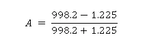
A = 0.998
For water- User Defined material RT instability,
ρ1 = 998.2 kg/m3 [Water density]
ρ2 = 400 kg/m3 [UD material density]
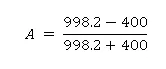
A = 0.428
Why Steady State simulation is not suitable ?
- We know that steady state simulation is a time independent approach.
- Based on the simulation we know there is high turbulence involve and the change in the flow occurs between very small time variation. This is not possible to capture in steady state solution
- Also steady state solver ignore the time differential terms involved in the simulation and thus even if it may be able to capture the state of equilibrium, it skips to capture the non-linearities in the simulation precisely.
CONCLUSION
- From the above cases, we observe that finer mesh captures the instability better than the coarse mesh, but it takes more time for the heavier fluid to settle down. As computational time is long but produces results with better accuracy.
- Since the simulation involves capturing instabilities that are changing in an unpredictable manner as a function of time, the transient approach is preferred over the steady-state approach.
- For Atwood number close to 0, RT instability flows take the form of symmetric fingers of fluid.
- when Atwood number close to 1, the much lighter fluid below the heavier fluid takes the form of larger bubble-like plumes.