Week 5 - Rayleigh Taylor Instability
Aim: Simulate Rayleigh Taylor Instability for 2 phase condition.
Theory:
Rayleigh Taylor Instability is an instability of an interface between 2 fluids of different densities, when lighter fluid pushes the heavier fluid or when lighter fluid accelerates intothe denser fluid. Some examples where this phenomenon is observed are formation of mushroom clouds due to volcanic erruptions, mushroom clouds from nuclear explosions, surface of expanding bubble in deepwaters.
When a heavier fluid is placed above a lighter fluid and made to fall under the influence of the gravity, the heavier fluids falls displacing the lighter fluid to lower its potential energy. Whereas, the lighter fluid is displaced at the same time increasing its potential energy but the toal energy of the system is lowered overall.
Saffman Taylor Instability (also known as viscous fingering):
It is observed during drainage process through media such as soils. It happens when a less viscous fluid displaces a more viscous fluid. Whereas in an inverse situation, flow of more viscous fluid displacing less viscous fluid, the interface is stable.
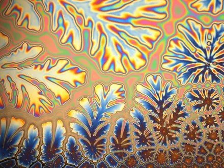
Viscous Fingering
Richtmyer Meshkov Instability:
RMI occurs when 2 fluids of different density are impulsively accelerated. When a shock wave impinges upon an interface seperating 2 gases having different densities on the either sides of the interface. The instability causes the perturbations on the interface to grow, producing vortical structures.
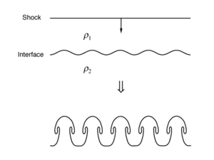
Richtmyer Meshkov Instability
Kelvin Helmholtz Instability:
The Kelvin–Helmholtz instability is a fluid instability that occurs when there is velocity shear in a single continous fluid or a velocity difference across the interface between two fluids. Kelvin-Helmholtz instabilities are visible in the atmospheres of planets and moons, such as in cloud formations on Earth or the Red Spot on Jupiter, and the atmosphere of the Suns and other stars.
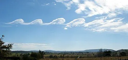
Kelvin Helmholtz Instability
Plateau Rayleigh Instability:
The Plateau–Rayleigh instability, often just called the Rayleigh instability, explains why and how a falling stream of fluid breaks up into smaller packets with the same volume but less surface area. This fluid instability is exploited in the design of a particular type of ink jet technology whereby a jet of liquid is perturbed into a steady stream of droplets.

Plateau-Rayleigh Instability
Atwood Number: It is a dimensionless number defined by `A=((rho_2-rho_1)/(rho_2+rho_1))`, where `rho_2`is density of the heavier fluid and `rho_1` is the density of the lighter fluid. It ranges between 0 & 1; and it is a measure of the instablity of the interface between the fluids. The higher the value of Atwood Number, more pronounded will be the instability of the interface and more longer time is required for it to stabilize.
Setup:
- Setting up case in Project Schematic
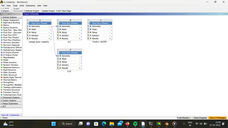
- Setting up Geometry
2 surfaces were created since its a 2D flow. The above layer being the heavier fluid with the reference being the gravity acting in the downward direction. Else there wont be any instability to begin with.
The interface i.e: common edge, is shared under workbench. If this is not done the interface is considered as a wall also no information will go across the interface.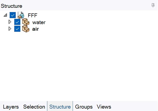
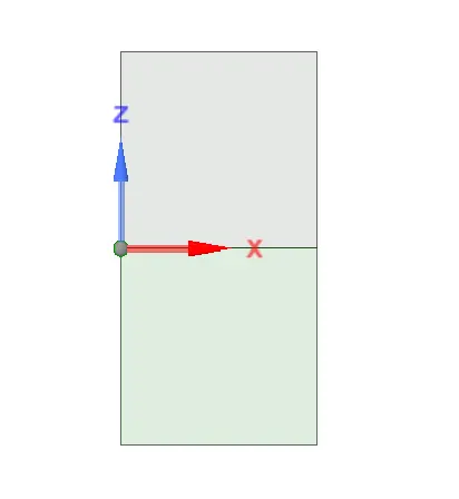
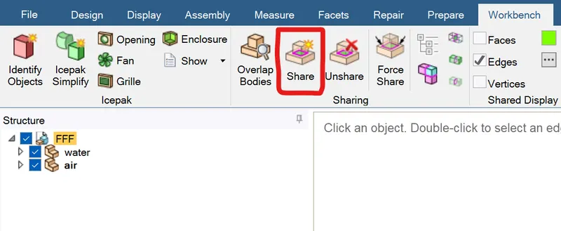
2 phase regions The geometry Sharing the common egde or interface - Meshing
Meshing was done with the element size of 0.5mm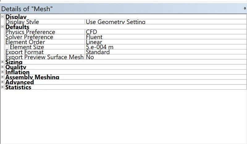
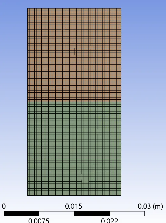
mesh data mesh
Other cases were ran with more refined mesh size as well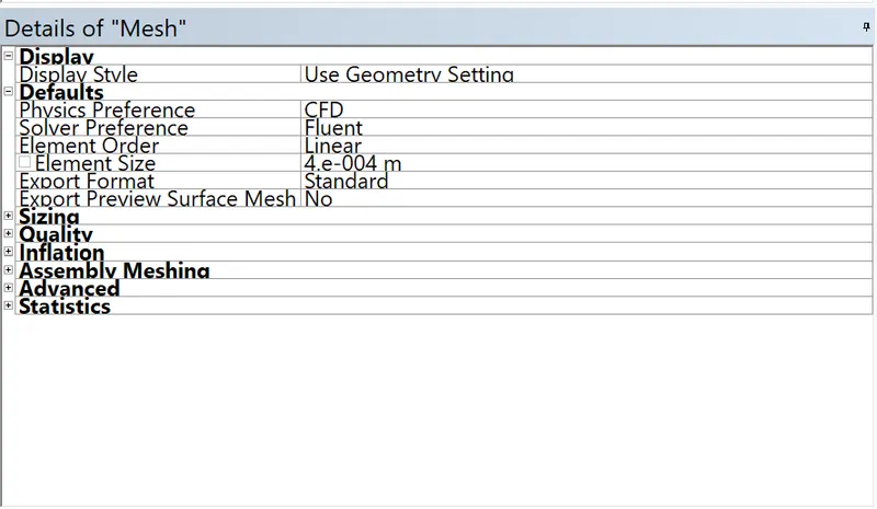
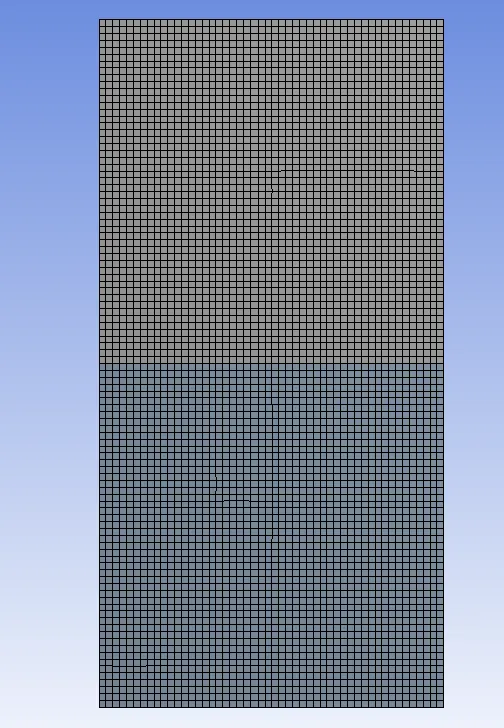
mesh data (0.4 mm) mesh (0.4 mm)
mesh data (0.25 mm) mesh (0.25 mm) - Solving:
As we are interested in how the flow develops rather than the final result, we choose the transient analysis.
The flow is incompressible hence pressure based solver.
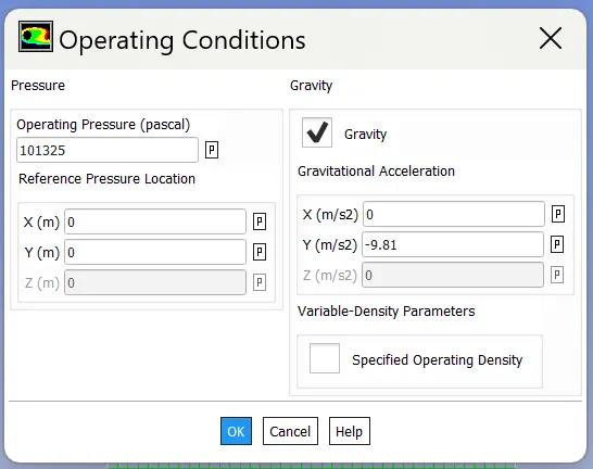
Gravity is introduced through operating conditions.
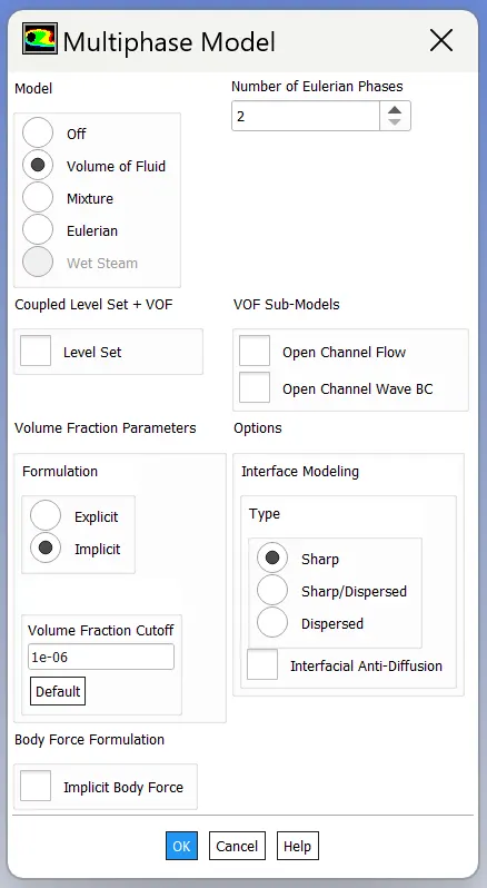
Volume of Fluid Method is chosen under multiphase model with implicit formulation. The case wwith explicit formulation was also used but were limited in their funtionalit. More on it on in the conclusion section.
Materials were defined (air and water). Another case was defined where air was replaced by another fluid with a density of 400 kg/m3 and viscosity of 0.001 kg/m-s.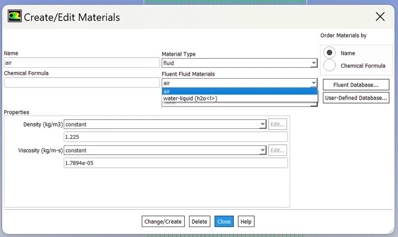
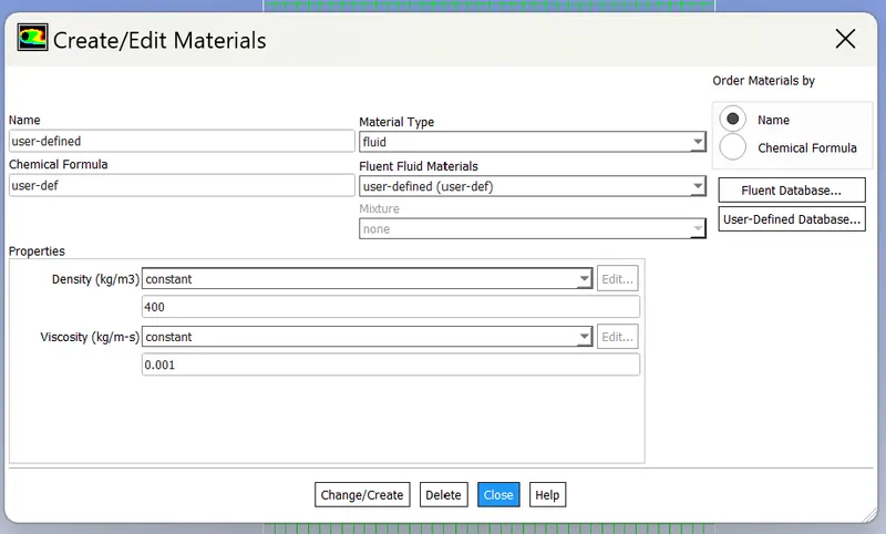
air & water water & a user defined material
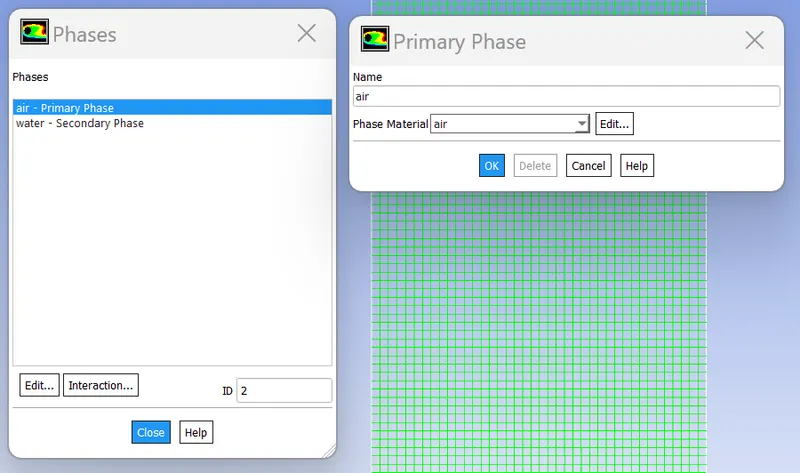
Phases are named and the fluids are assigned to each of the phases
- Initialization & solving:
The simulation is initialized. The initialization used is standard initialization.
After initizlizing the solution we have to patch the flow variables. Patch is used to assign different values of particular variables into different cells. In our case we use patch because we need to assign different value of Volume fraction to two different fluids.
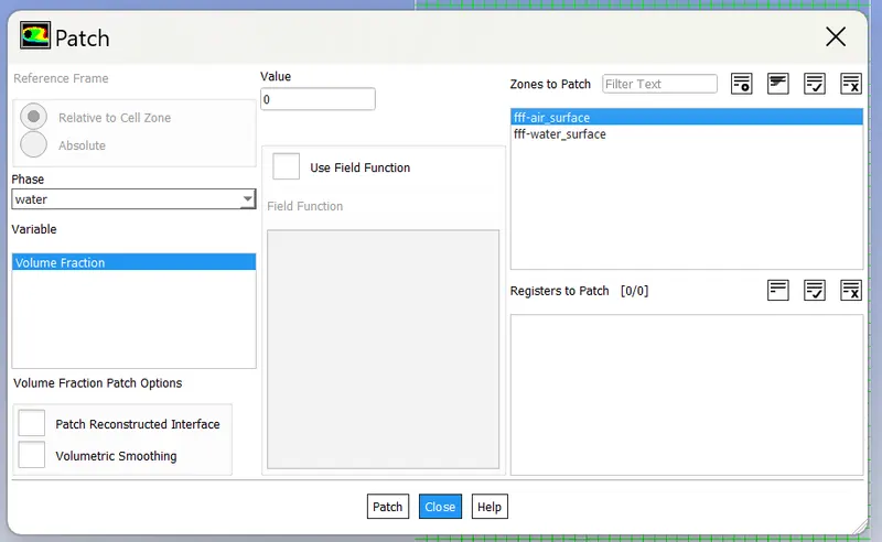
The contour plot and animation file is created followed by running the simulation for a given time step size and a given number of iterations.
Results:
- The animations for these cases were obtained and the links for the same are attached in the report.
- The interface breaks instantly with heavier fluid intruding into lighter fluid phase, at the same time the lighter fluid also protruding into heavier fluid region at a different location forming a mushroom cloud like structure.
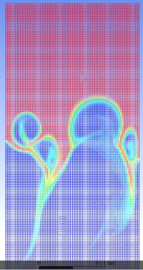
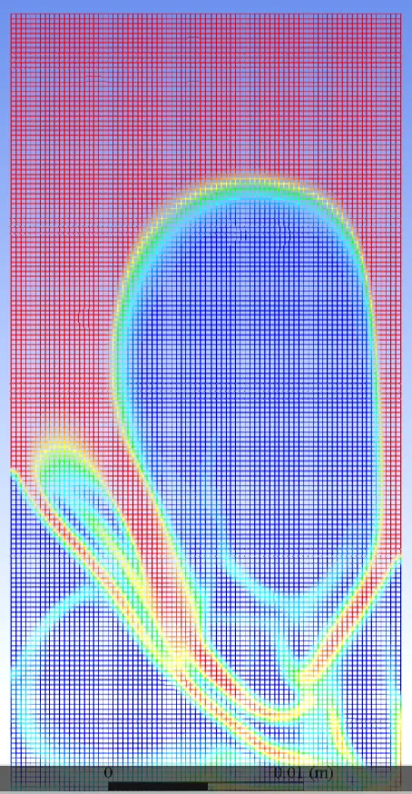
As the simulation progresses the mixing gets more pronounced with multiple interfaces being formed and merged until the heavier fluid and lighter fluid swap their initial position entirely. - One more observation was that the intial interface which was a line, now is a continous region wih voulme fraction value between 0 and 1. However, this eventually goes back to form a line interface but it happens slowly and takes a comparitively longer time.
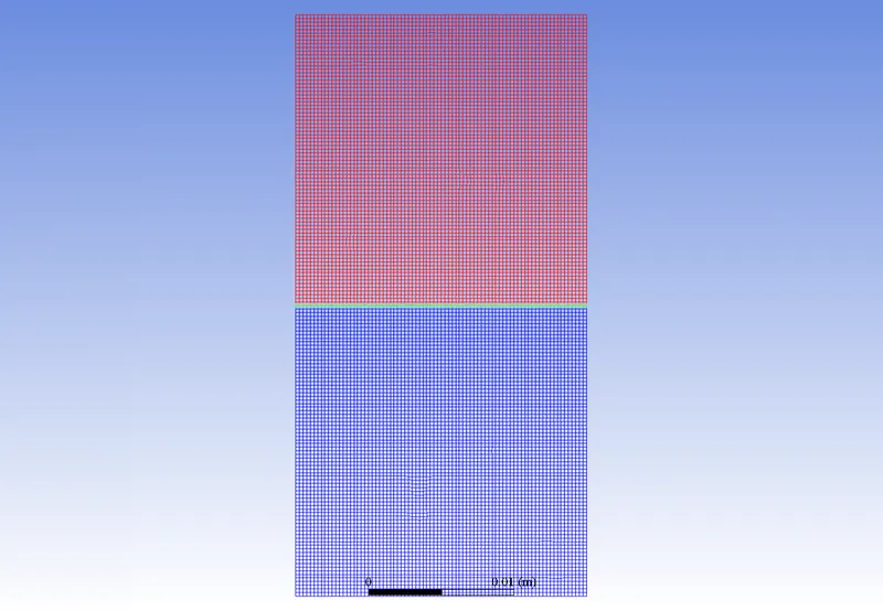
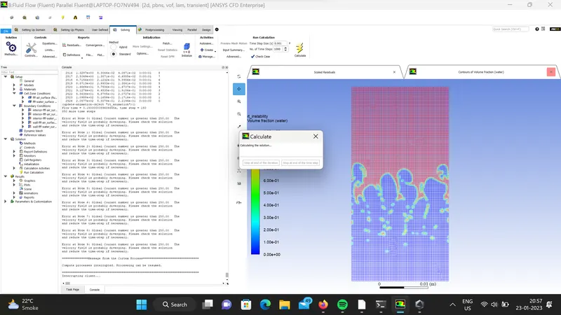
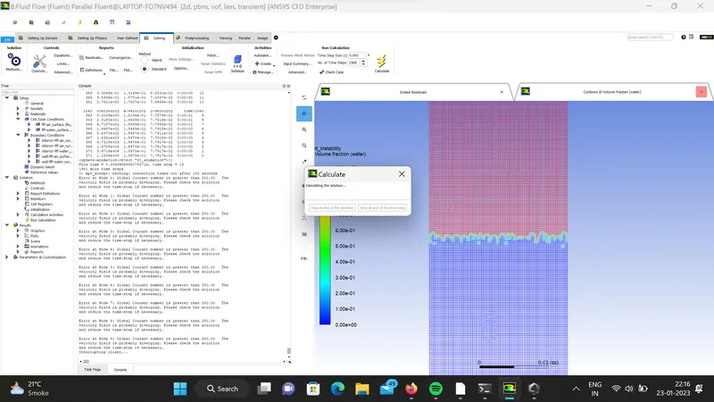
- The explicit method posed few problems which makes this method as not the best choice for transient multiphase simulation. The number of iterations required is large and still stability isn't certain.
- Atwood number (A) for water-air case is 0.997, for water-user defined fluid case Atwood number is 0.427.
- The case with the water and fluid with density of 400 kg/m3, the plume or bubble formation is less pronounced than the case of water-air case.
Conclusion:
- The higher the Atwood Number, greater will be the instability of the interface. Same can be verified with the simulation results. The closer the Atwood number is to 1 more unstable the interface of the fluids will be. The closer the Atwood number is to 0, the lesser will be the unstability.
- When Atwood number is equal to 0, there is no stability of the interface.
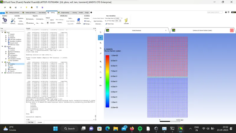
- The explicit method places a condition for choosing time step value for a given grid size. The condition is Courant number < 0.5. This plus the fact that, we dont have velocity information and how it changes over the simulation period which makes deciding upon the time step value even more difficult. As shown below even a time step as low as 0.005 and 0.0001 results in diverging of the solution.
- Even if we take a conservative approach and assume a probable velocity value using `v=sqrt(2gh)`, the time step value is very small which makes the simulation time very long. Hence, implicit scheme seems a better choice for performing multiphase simulation.
- A steady state approach is not suitable for such simulation because we are more interested in dynamic behavior of the interface between the fluids rather than the steady state results which is already known.
Animation Links:
https://drive.google.com/file/d/1krILlZbYgRC2qVdL4uuLS5cUVigvUE_B/view?usp=sharing
https://drive.google.com/file/d/1-Zn8kneCeEaawzby6GGGmUKOP00em1Rm/view?usp=sharing
https://drive.google.com/file/d/1W98jr1Ugptb6qXJKeh56RrspuwoiLomh/view?usp=sharing