Week 5 - Rayleigh Taylor Instability

Aim:

to perform the rayleigh taylor instability between two different immiscible liquids with two different mesh sizes and discuss the consequences

Objectives:

1. What are some practical CFD models that have been based on the mathematical analysis of Rayleigh Taylor waves? In your own words, explain how these mathematical models have been adapted for CFD calculations.
2. Perform the Rayleigh Taylor instability simulation for 2 different mesh sizes with the base mesh being 0.5 mm. Compare the results by showing the animations( Attach them from your google drive). Observe the differences in the animation and explain the effect of mesh size on simulation. Also, explain why a steady-state approach might not be suitable for these types of simulation.[ Choose Air and Water for this simulation]
3. Run one more simulation with water and user-defined material(density = 400 kg/m³, viscosity = 0.001 kg/m-s) for refined mesh.
4. Define the Atwood Number. Find out the Atwood number for both the cases and explain how the variation in Atwood number in the above two cases affects the behavior of the instability.

Rayleigh taylor instability:

Rayleigh-Taylor instability (RTI) is the interpenetration of materials that occurs whenever a light fluid pushes on a heavy fluid (Rayleigh 1883, Taylor 1950). It is a dynamic process whereby the two fluids seek to reduce their combined potential energy.

common example of such occasions in water over oil .

Practical CFD models that have been based on mathematical analysis of RT waves...

1. Kelvin-Helmholtz instability
2. Richtmyer-Meshkov instability
3. Plateau-Rayleigh instability

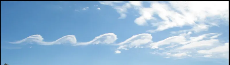
Kelvin-Helmholtz instability- This instability typically occurs when there is velocity shear in a single continuous fluid, or additionally where there is a velocity difference across the interface between two fluids. A common example is seen when wind blows across a water surface; the instability constant is able to manifest itself through waves on water surface. The Kelvin-Helmholtz instability is not only restricted to a water surface as clouds, but is evident through other natural phenomena as ocean and the sun's corona.

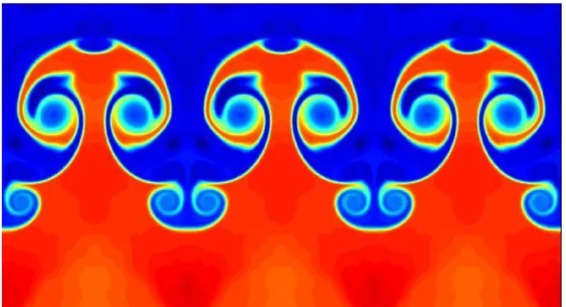
Richtmyer-Meshkov instability- This occurs when two fluids of different density are impulsively accelerated. Normally this is by the passage of a shock wave. The development of the instability begins with small amplitude perturbations which initially grow linearly with time. This is followed by a nonlinear regime with bubbles appearing in the case of a light fluid penetrating a heavy fluid, and with spikes appearing in the case of a heavy fluid penetrating a light fluid. A chaotic regime eventually is reached and the two fluids mix. This instability can be considered the impulsive-acceleration limit of the Rayleigh Taylor instability.

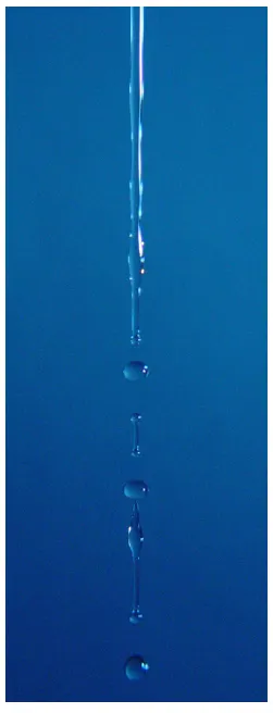
Plateau-Rayleigh instability- This instability, often just called the Rayleigh instability, explains why and how a falling stream of fluid breaks up into smaller packets with the same volume but less surface area. It is related to the RTI and is part of a greater branch of fluid dynamics concerned with fluid thread breakup. This fluid instability is exploited in the design of a particular type of ink jet technology whereby a jet of liquid is perturbed into a steady stream of droplets. The driving force of the Plateau–Rayleigh instability is that liquids, by virtue of their surface tension, tend to minimize their surface area.

Approach:

1. creating geomentry in space claim
2. meshing
3. fluent setup
4. cfd post

1. creating geomentry in space claim:

open space claim and create structure in XY plane like shown.

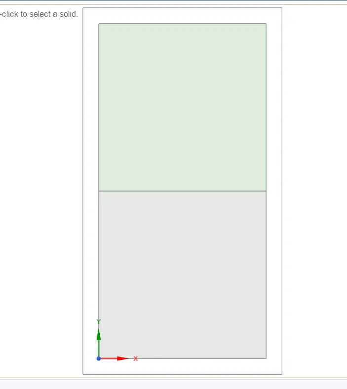
both the parts are 20sq dimension and named as heavier and lighter component respectively and also make it to share topology as shown

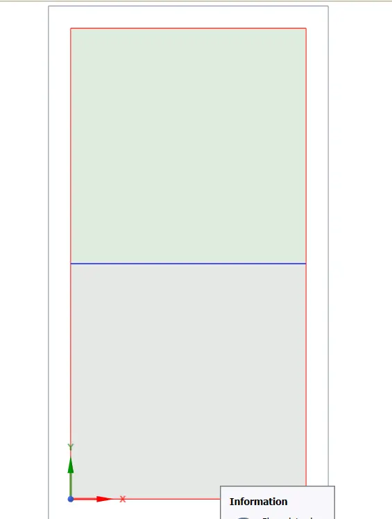
blue colour line represents shared lines while sharing topology between two surfaces.

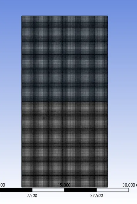
first we need to create base mesh of size 0.5mm

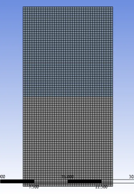
open solvent ansys fluent:

set as viscous -laminour flow with multiphasemodel of two phases air and water as materials

also turn on gravity

initialize the simulation and also use patch options for showing contour in both solids as well

we need to create animate file of changing watrer and air

after initializing patch two different phases with fraction percentage of water

run simulation for 0.005 sec time step for 500 time steps.

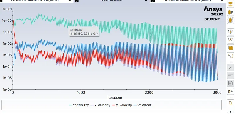
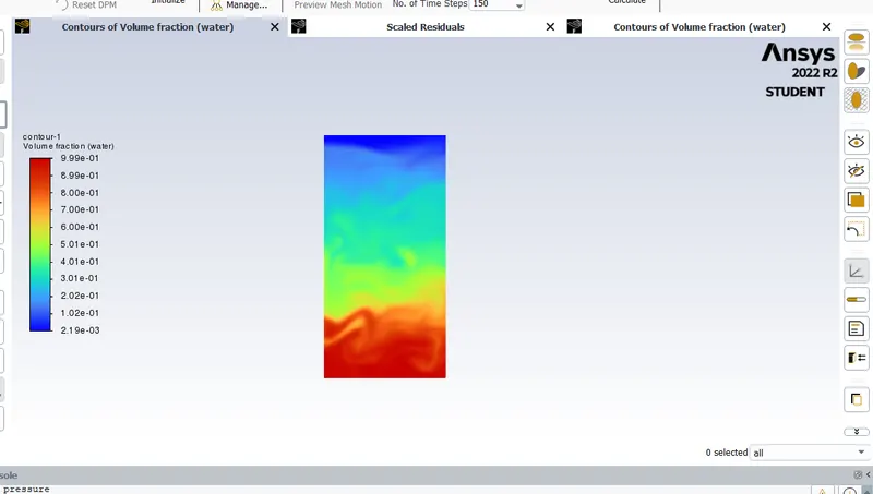
also refer to the animated file refer link

https://drive.google.com/file/d/14CLJpv7rdgZSzu3CvVQwNSXSkiC8zfVT/view?usp=share_link

in this case we can observe bubble formation slowly

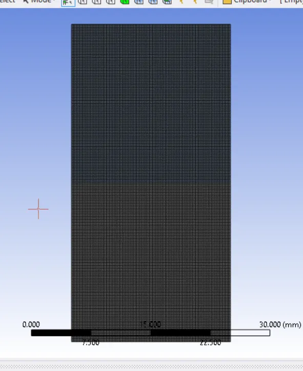
also by duplicating files in work bench perform simulation for two differnt meshes of size 0.25 mm mesh and 0.2mm mesh sizes for same setup

0.25mm mesh sizes

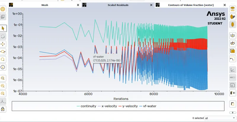
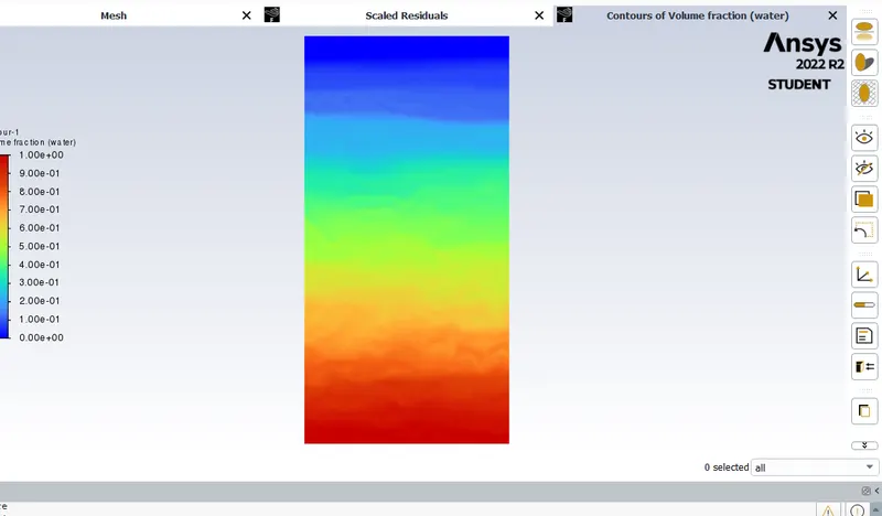
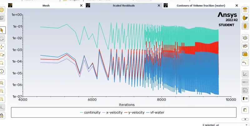
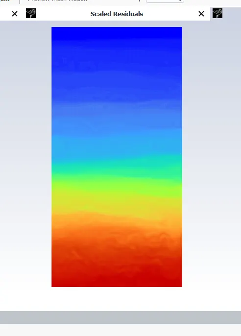
animated file link: https://drive.google.com/file/d/1isX-pbp82Wx9Kvwi-uaItH5pQOVy8cuV/view?usp=share_link

in this case we can see quiet formation of bubbles more precisely

case 2:

repeat the simulation with same mesh size but instead of air use material with 400 kg/m3 density and 0.01kg/m-sec viscosity

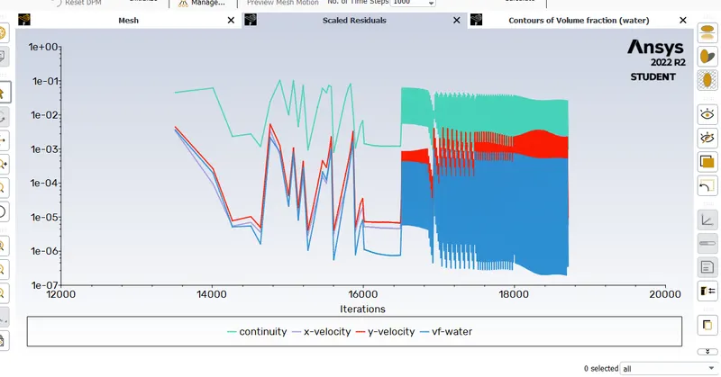
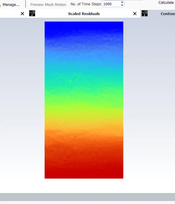
animation file link : https://drive.google.com/file/d/1tHF6qEj62OrVgcTpWw8lDHr9GvBvfB5I/view?usp=share_link

Atwood number:

The Atwood number (A) is a dimensionless number in fluid dynamics used in the study of hydrodynamic instabilities in density stratified flows. It is a dimensionless density ratio defined as

where

�1 = density of heavier fluid

�2 = density of lighter fluid

ok lets discus the both cases we solved above

case1:

density of water d1= 998.2 kg/m3

density of air d2= 1.225 kg/m3

then atwood number be A= (998.2 -1.225)/(998.2 + 1.225)

A = 0.9975

case 2:

density of water d1= 998.2 kg/m3

density of material d2= 400 kg/m3

A= (998.2 - 400)/(998.2 + 400) = 0.427

A=0.427

Atwood no close to 1 indicates the bubble formation, and value close to 0 indicates wake like formation without any bubble.

Conclusion:

• The finer the mesh, the more correct the observation of bubble formation can be captured.
• Incorrect time steps or large courant no can lead to floating point errors. So required relaxation factors should be given accordingly.
• With increase in mesh refinement, the computational time increases.
• The Atwood no validates the CFD simulation as it is observed. In case of water and air mixing, bubble formation takes place, whereas for the other case no bubble takes place.