Week 5 - Rayleigh Taylor Instability
Aim:
- To Perform the Rayleigh Taylor instability simulation for 2 different mesh sizes with the base mesh being 0.5 mm and to Compare the results by showing the animations
- To Observe the differences in the animation and explain the effect of mesh size on simulation. Also, explain why a steady-state approach might not be suitable for these types of simulation.[ to consider Air and Water for this simulation]
- To Run one more simulation with water and user-defined material(density = 400 kg/m3, viscosity = 0.001 kg/m-s) for refined mesh.
- To Define the Atwood Number and Find out the Atwood number for both the cases and explain how the variation in Atwood number in the above two cases affects the behavior of the instability.
Introduction:The Rayleigh–Taylor instability, or RT instability is an instability of an interface between two fluids of different densities which occurs when the lighter fluid is pushing the heavier fluid.Examples include the behavior of water suspended above oil in the gravity of Earth, mushroom clouds like those from volcanic eruptions and atmospheric nuclear explosions, supernova explosions in which expanding core gas is accelerated into denser shell gas, instabilities in plasma fusion reactors and inertial confinement fusion.Water suspended atop oil is an everyday example of Rayleigh–Taylor instability, and it may be modeled by two completely plane-parallel layers of immiscible fluid, the denser fluid on top of the less dense one and both subject to the Earth's gravity. The equilibrium here is unstable to any perturbations or disturbances of the interface: if a parcel of heavier fluid is displaced downward with an equal volume of lighter fluid displaced upwards, the potential energy of the configuration is lower than the initial state. Thus the disturbance will grow and lead to a further release of potential energy, as the denser material moves down under the (effective) gravitational field, and the less dense material is further displaced upwards.
Hydrodynamics simulation of a single "finger" of the Rayleigh–Taylor instability RT instability fingers evident in the Crab Nebula
Practical CFD models that have been based on mathematical analysis of RT waves.
The Kelvin–Helmholtz instability is a fluid instability that occurs when there is velocity shear in a single continuous fluid or a velocity difference across the interface between two fluids. Kelvin-Helmholtz instabilities are visible in the atmospheres of planets and moons, such as in cloud formations on Earth or the Red Spot on Jupiter, and the atmospheres of the Sun and other stars.
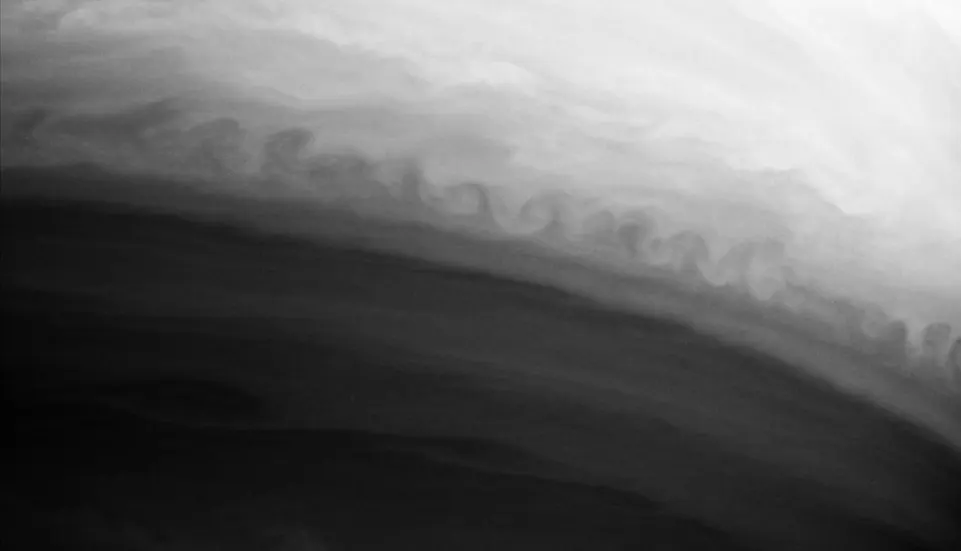
A KH instability on the planet Saturn, formed at the interaction of two bands of the planet's atmosphere.
The Richtmyer–Meshkov instability (RMI) occurs when two fluids of different density are impulsively accelerated. Normally this is by the passage of a shock wave. The development of the instability begins with small amplitude perturbations which initially grow linearly with time. This is followed by a nonlinear regime with bubbles appearing in the case of a light fluid penetrating a heavy fluid, and with spikes appearing in the case of a heavy fluid penetrating a light fluid. A chaotic regime eventually is reached and the two fluids mix. This instability can be considered the impulsive-acceleration limit of the Rayleigh–Taylor instability.
The Plateau–Rayleigh instability, often just called the Rayleigh instability, explains why and how a falling stream of fluid breaks up into smaller packets with the same volume but less surface area. It is related to the Rayleigh–Taylor instability and is part of a greater branch of fluid dynamics concerned with fluid thread breakup. This fluid instability is exploited in the design of a particular type of ink jet technology whereby a jet of liquid is perturbed into a steady stream of droplets.
The driving force of the Plateau–Rayleigh instability is that liquids, by virtue of their surface tensions, tend to minimize their surface area. A considerable amount of work has been done recently on the final pinching profile by attacking it with self-similar solutions.
Procedure:
step 1: open ansys workbench and click on geometry and open space claim, create square of 20mm in xy plane and perform pull for creating surfaces and rename the sketch as air,next
create new sketch of square of 20mm in same xy plane on top of first surface and rename it as water.
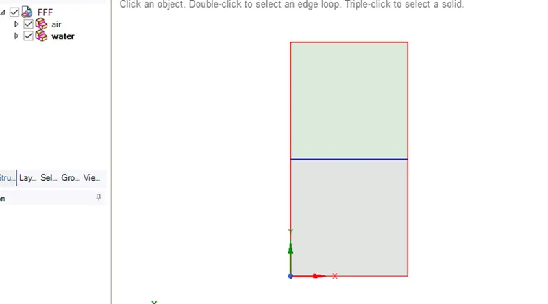
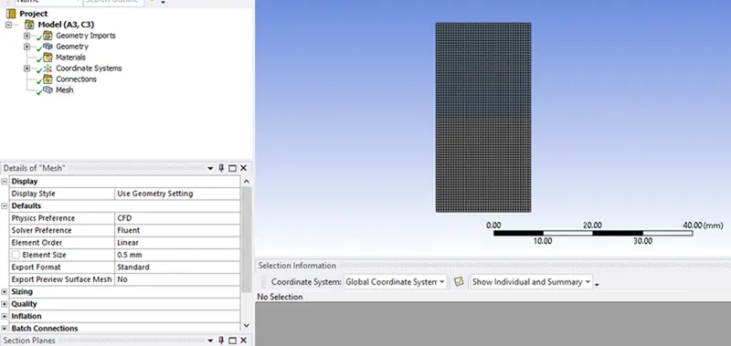
step 2: open mesh, create a base mesh of element size = 0.5mm and check the quality criteria and close
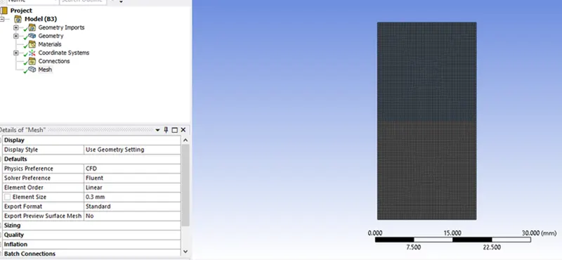
for case 2= mesh element size= 0.3mm
step3: open setup fluent, follow the below points for both the cases and analyze the solution.
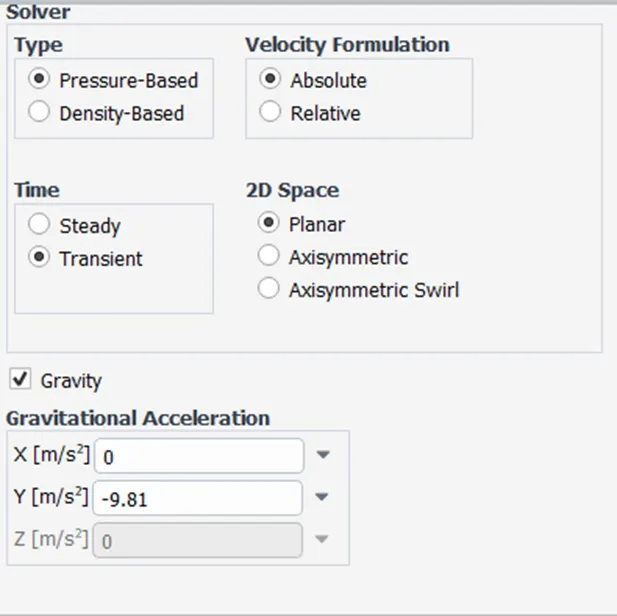
- under general->select transient(since we are conducting simulation with respect to function of time and also due to instability)->pressure based->absolute velocity->click on gravity(the denser fluid on top of the less dense one and both subject to the Earth's gravity)->y coordinate=-9.81m/s.
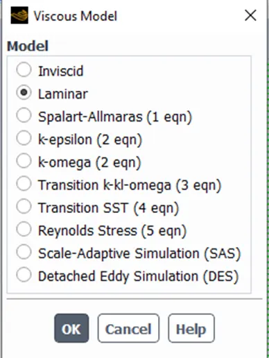
- viscous model->laminar
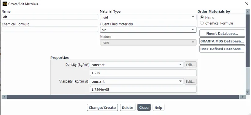
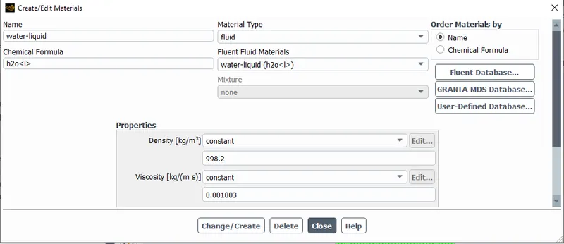
- under material choose the two fluids as air and water for first two cases and for the special case create user materail by clicking fluent database->air->copy->change name to material-new->ok, with density= 400kg/m^3;viscosity=0.001 kg/m-s
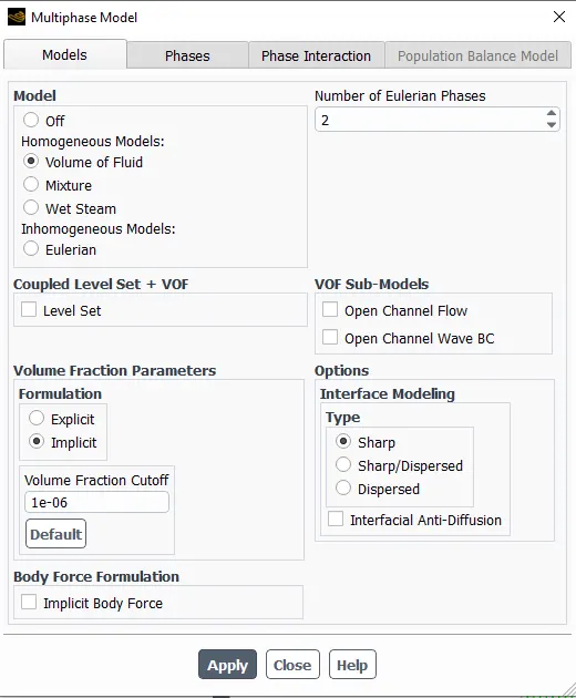
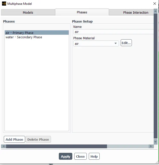
- under multiphase select fluid volume method->volume fraction parameters formulation is implicit->no of eulerian phases= 2->ok, next under phase select primary phases as air and secondary phase as water.
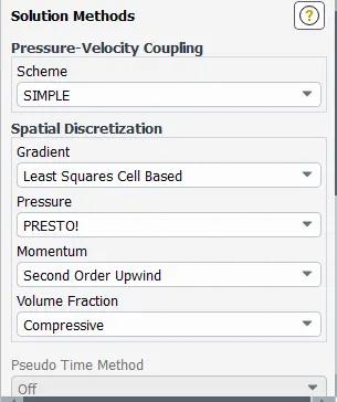
- choose the method as simple as we are dealing with laminar
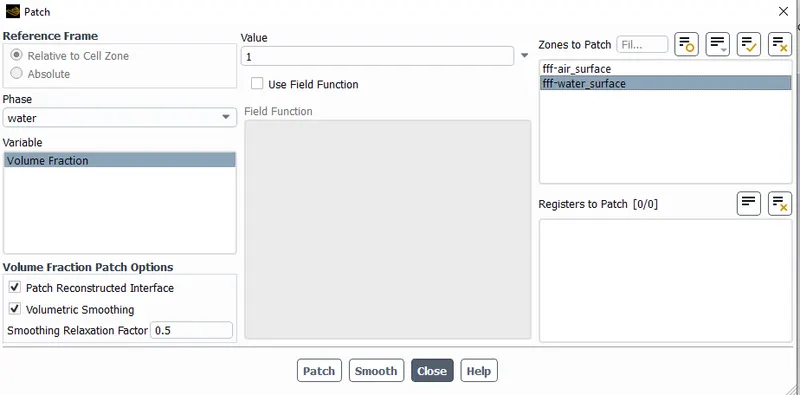
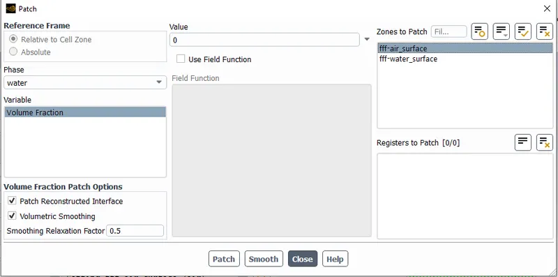
- initialize the solution using the standard method and patch the model, for air give the alpha value as 0 and water as 1.
- create a contour for the phases and also the animation for the volume fraction of water.
- Now run the simulation with a time step size of 0.025 and 100 no. of iteration. if we encounter any error while running the simulation try reduce the mesh size and run the simulation again.
Results:
Case 1: Basemesh with an elemental size = 0.5mm and having the fluid materials air and water.
elements=2888
timestep size=0.025
no. of iteration=600
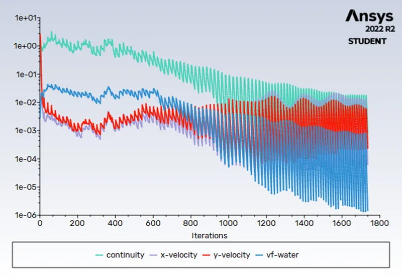
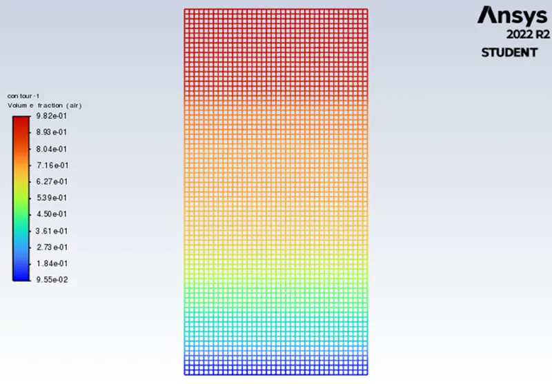
residuals volume fraction contour
Case 2: refined mesh with an elemental size o= 0.3 mm and having the fluid materials air and water.
elements=7938
timestep size=0.001
no. of iteration=600
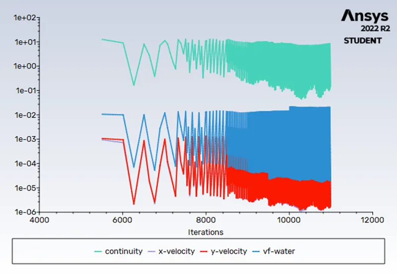
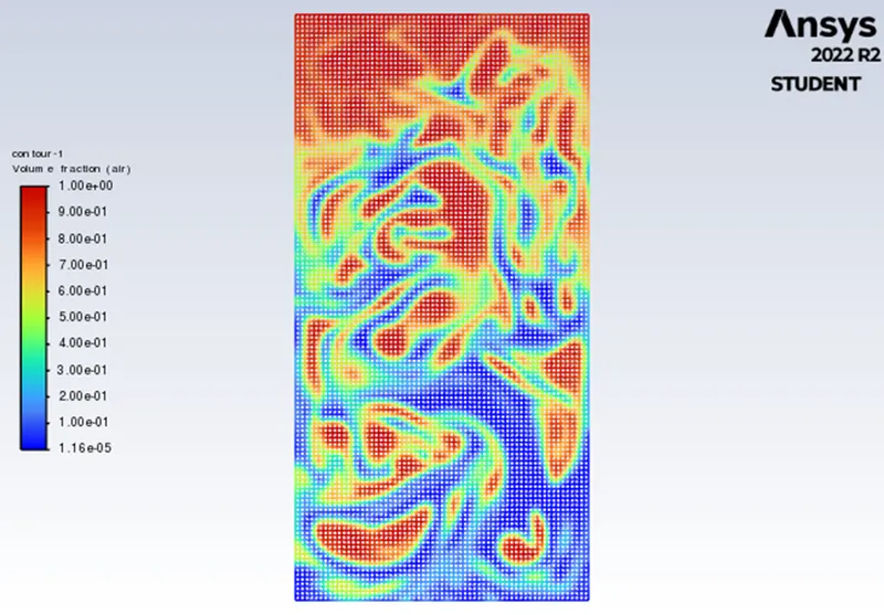
residuals volume fraction contour
Case 3: refined mesh with an elemental size o= 0.5 mm and having the fluid materials user material(materail-new) and water
elements=2888
timestep size=0.005
no. of iteration=600
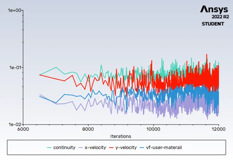
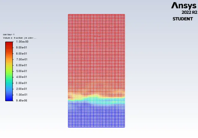
residuals volume fraction contour
explain why a steady-state approach might not be suitable for these types of simulation.
The steady-state analysis study holds good for final result. But here in this study, the instabilities information is sensitive and time-dependent and is growing exponentially at each time step. Steady-state simulation can capture those instabilities but the results will not be time-dependent. but Transient simulation with reduced time-steps can capture these instabilities at each and every time-steps and time-dependent results can be obtained as we know that transient simulation is done as a function of time.
4. Atwood number (A)
The Atwood number (A) is a dimensionless number in fluid dynamics used in the study of hydrodynamic instabilities in density stratified flows. It is a dimensionless density ratio defined as

where
 = density of heavier fluid
 = density of lighter fluid
- The difference in the fluid densities divided by their sum is defined as the Atwood number A.
Case 1 & 2:For fluid materials air and water
ρ1=density of water=998.2kg/m^3
ρ2=density of air=1.225kg/m^3
A=998.2-1.225/(998.2+1.225);
A=0.9975
Case 3:For fluid materials user defined and water
ρ1=density of water=998.2kg/m^3
ρ2=density of user defined=400kg/m^3
A=998.2-400/(998.2+400);
A=0.427
Higher the Atwood Number, more the instability between the fluids, therefore in case 1& 2 with higher atwood number we can see that the lighter fluid penetrate the heavier fluid as bubbles, while the spikes of the heavier fluid move into the lighter fluid.The change in Atwood number, has a direct impact on the amplitude perturbation region and impacts on the variation of interface growth. using the fluid volume method of finer mesh and smaller time-steps gave promising visualization of Rayleigh-Taylor instability.
conclusion:
- the Rayleigh Taylor instability simulation for 2 different mesh sizes with the base mesh being 0.5 mm were performed and also Compared the results by showing the animations
- Observed the differences in the animation and explained the effect of mesh size on simulation. Also, explained why a steady-state approach might not be suitable for these types of simulation.
- one more simulation with water and user-defined material(density = 400 kg/m3, viscosity = 0.001 kg/m-s) for refined mesh were conducted and observed.
- the Atwood Number were defined and the Atwood number for both the cases were found out and explained how the variation in Atwood number in the above two cases affects the behavior of the instability.
references link: