Week 5 - Rayleigh Taylor Instability

• Rayleigh Taylor Instability
  1. What are some practical CFD models that have been based on the mathematical analysis of Rayleigh Taylor waves? In your own words, explain how these mathematical models have been adapted for CFD calculations.
  2. Perform the Rayleigh Taylor instability simulation for 2 different mesh sizes with the base mesh being 0.5 mm. Compare the results by showing the animations( Attach them from your google drive). Observe the differences in the animation and explain the effect of mesh size on simulation. Also, explain why a steady-state approach might not be suitable for these types of simulation.[ Choose Air and Water for this simulation]
  3. Run one more simulation with water and user-defined material(density = 400 kg/m³, viscosity = 0.001 kg/m-s) for refined mesh.
  4. Define the Atwood Number. Find out the Atwood number for both the cases and explain how the variation in Atwood number in the above two cases affects the behavior of the instability.
• Aim- To conduct the Rayleigh Taylor CFD simulation
• Objective - To Perform the Rayleigh Taylor instability simulation for 2 different mesh sizes with the base mesh being 0.5 mm.
• To compare the results by showing the animations( Attach them from your google drive). Observe the differences in the animation and explain the effect of mesh size on simulation. Also, explain why a steady-state approach might not be suitable for these types of simulation.

• Atwood number
• The Atwood number (A) is a dimensionless number in hydrodynamics used in the study of hydrodynamic instabilities in densely stratified flows. It is a dimensionless density ratio defined as:

where , = density of heavier fluid

= density of lighter fluid

• Atwood number is an important parameter in the study of Rayleigh–Taylor instability
• Courant number -The one-dimensional courant number is defined as C ≡ u∆t/ ∆x. where u is the characteristic wave velocity of the system, ∆t is the time step of the numerical model, and ∆x is the grid spacing of the numerical model. .

• What are some practical CFD models that have been based on the mathematical analysis of Rayleigh Taylor waves? In your own words, explain how these mathematical models have been adapted for CFD calculations.
• The Rayleigh–Taylor instability is a fundamental instability of an interface between two fluids of different densities, which occurs when the light fluid is pushing the heavy fluid.
• During the nonlinear stages, the growth of the Rayleigh–Taylor instability is greatly affected by three-dimensional effects.
• Water suspended atop oil is an everyday example of Rayleigh–Taylor instability, and it may be modeled by two completely plane-parallel layers of immiscible fluid, the denser fluid on top of the less dense one and both subject to the Earth's gravity.
• Examples include the behavior of water suspended above oil in the gravity of Earth,mushroom clouds like those from volcanic eruptions.
• Practical CFD Models
  
  SPH Method (Smoother Particle Hydrodynamics)
  
  Smoothed-Particle Hydrodynamics (SPH) is a computational method for simulating the dynamics of continuous media, such as solid mechanics and fluid flow. Smoothed particle hydrodynamics is increasingly used to model fluid motion. This is because it offers several advantages over traditional grid-based techniques. First, SPH guarantees mass conservation without additional computations, since the particles themselves represent the mass. Second, SPH computes pressure from weighted contributions from neighboring particles rather than solving a system of linear equations. Finally, unlike grid-based techniques, which need to track fluid boundaries, SPH directly creates free surfaces for two-phase interacting fluids. This is because particles represent dense fluids and spaces represent lighter fluids.
• SINGLE-FLUID MODEL
  A typical approach to the analysis of two-phase flow is the mixing model. That is, the individual fluid phases behave like flowing mixtures described by the mixture properties. The one-fluid model applied is a five-equation model consisting of the mass, momentum, and energy equations for the gas-liquid mixture and two equations describing the formation and growth of the liquid phase.
• Two-liquid model
  The two-liquid model used separate governing equations for the gas and liquid phases. Interactions between droplets and heat exchange between liquid and solid boundaries are also not modeled here. In addition, the model takes into account the velocity slip between the gas and liquid phases.
• Turbulence Models
  Turbulence models are required to predict the average mixing behavior of one or two dimensional average inflows. Approaches to building tile turbulence models are based on experimental behavior

• Procedure
• Draw 2 squares one above the other with a length of 0.02 m.
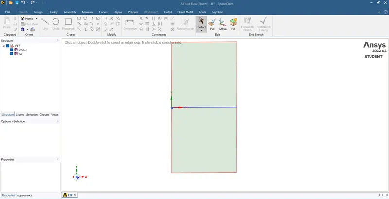
• Then naming the below square as air and above square as water in 2 different components.
• 

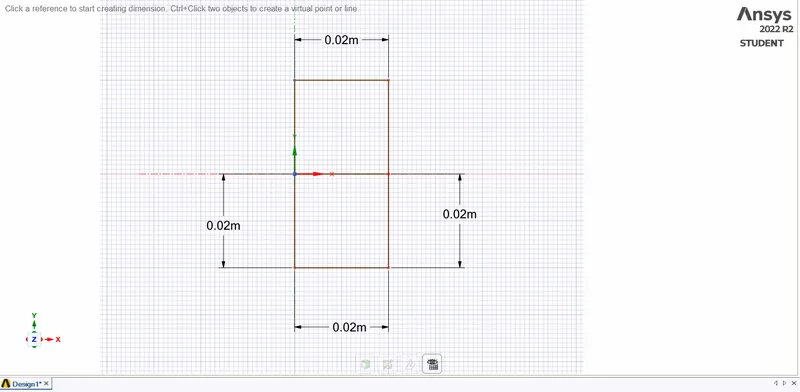
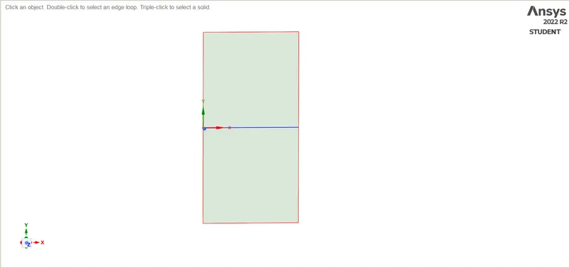
• Create surfaces and do share topology

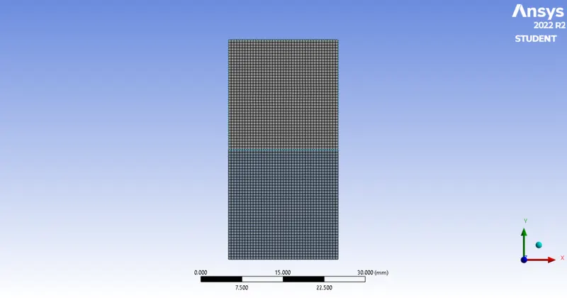
• Meshing with element size 0.5 mm

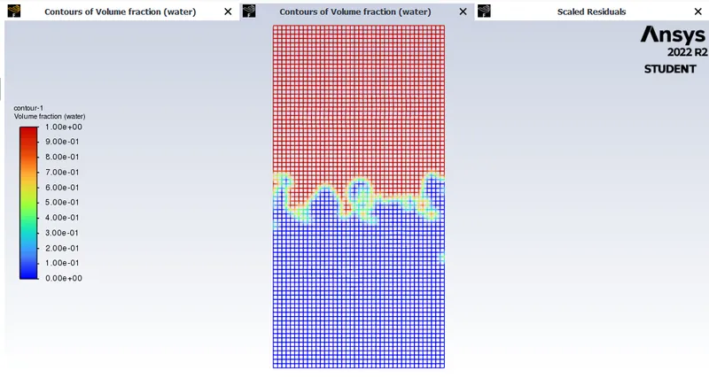
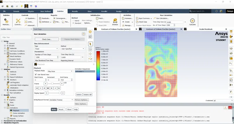
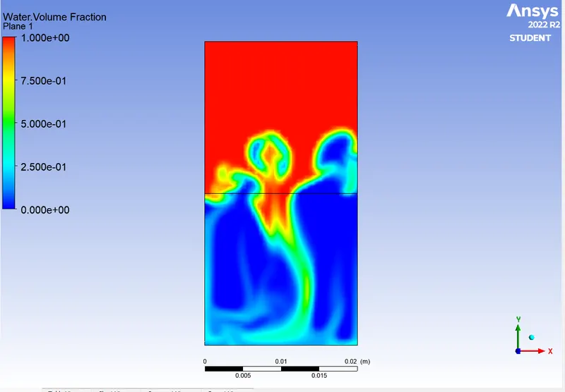
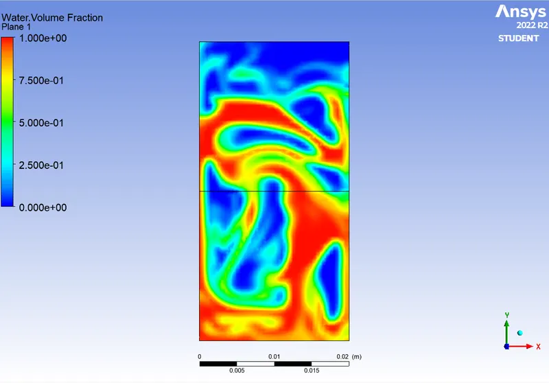
• Results - case 1
• Time step size = 0.005
• Timesteps = 1500

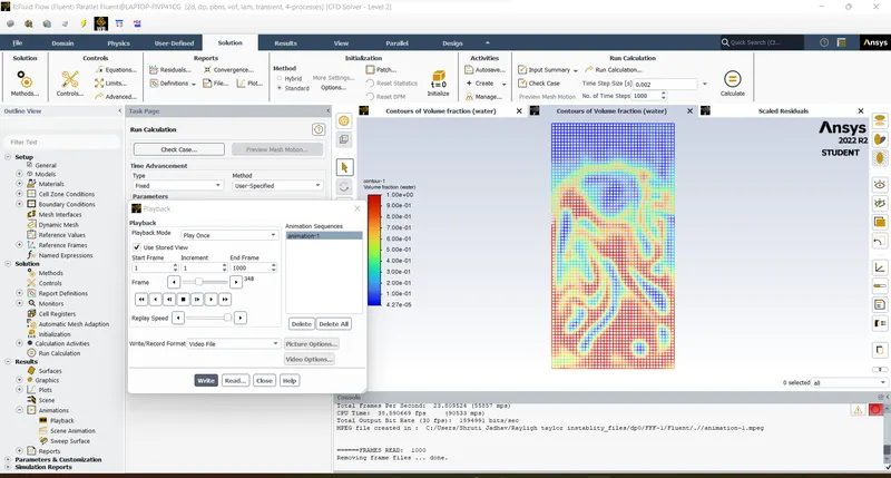
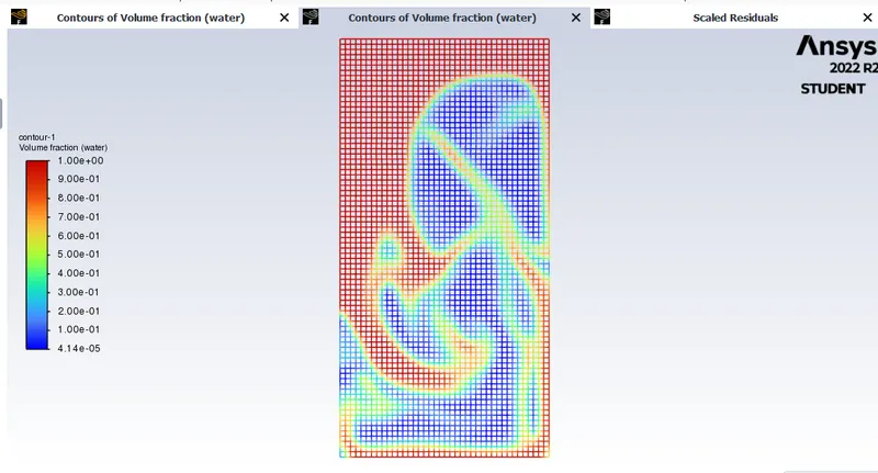
• Time step size = 0.002

• Residuals

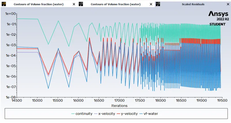
Link uploaded on youtube - https://youtu.be/pq0Jp4rQ13Y

• Case 2

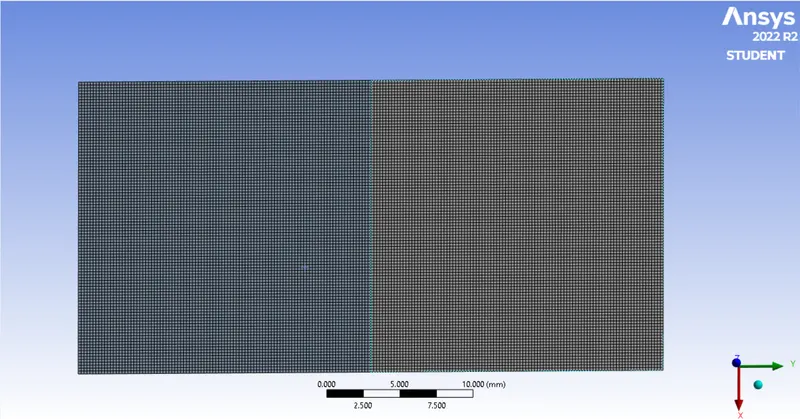
• Refined mesh

  Mesh properties:

  Element size = 0.2 mm

  Statistics:

• Mesh

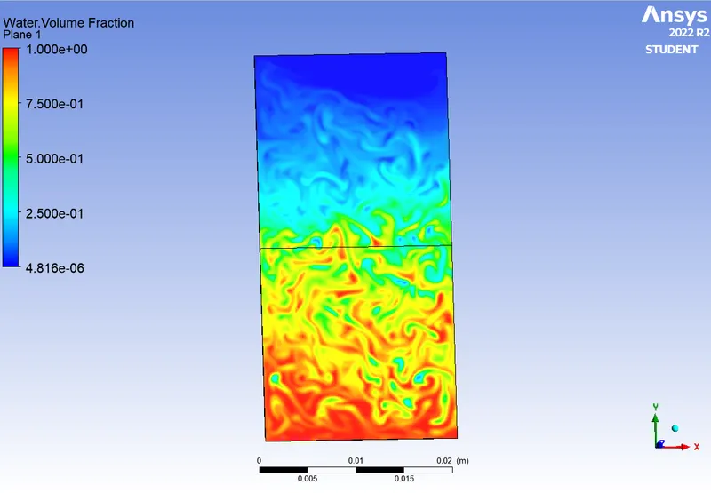
• Results

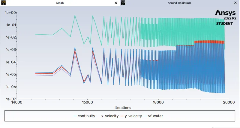
• Residuals

Link uploaded on youtube: https://youtu.be/c4uOEPxlVm0

• Run one more simulation with water and user-defined material(density = 400 kg/m³, viscosity = 0.001 kg/m-s) for refined mesh.

• CASE 3 -

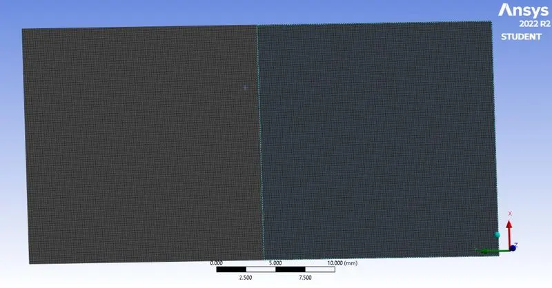
  STEP 3: MESH

  Overall Element size: 0.1 mm

• SETUP
  Solver Type	Pressure-Based
  Velocity Formulation	Absolute
  Time	Un-Steady
  Models	Viscous model: laminar Multiphase: Volume of fluid : Implicit formulation : 2 phases
  Material	Fluid type: User-defined-fluid(Density =400 kg/m3, viscosity = 0.001 kg/m-s) : water liquid Solid-type: Aluminium
  Cell zones	Fluid type: Air : water
  Boundaries	Standard
  Reference values	Standard
  Initialization	Standard Patch: Water-surface (1 value of volume fraction of water) : Air-surface(0 value of volume fraction of water)

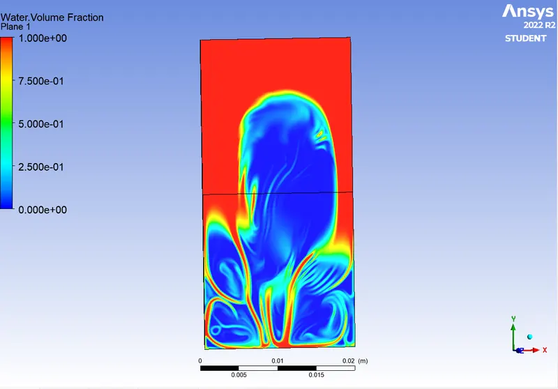
• Volume Fraction

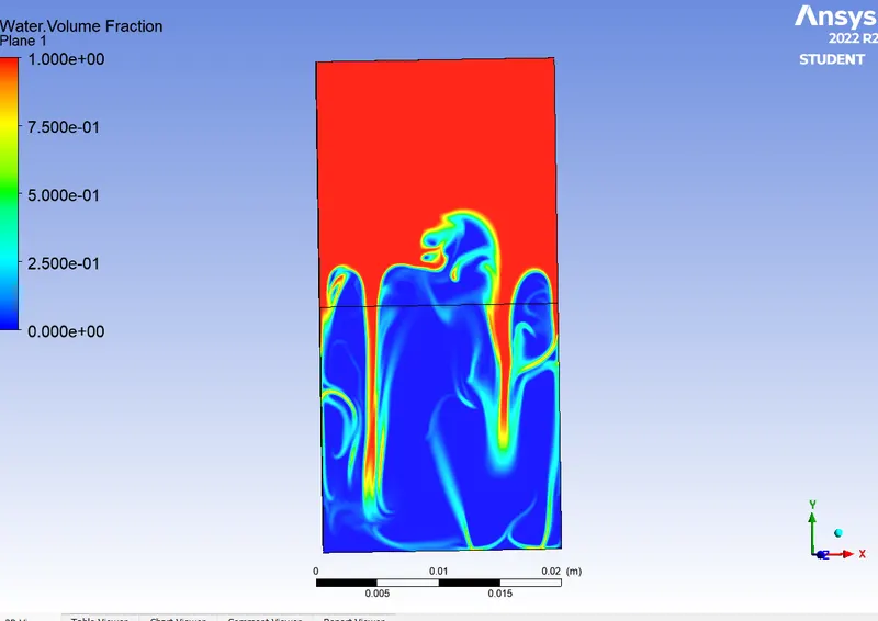
• Residuals

Link uploaded on youtube: https://youtu.be/vwTgHnd_dlI

• Stepwise Explaination
• This project considers three different cases. Two cases are based on MESHING types and the other one uses a custom material.
• Superimpose two substances, air and water, and see the effect of gravity on them.
• Draw two squares of length 0.02 m superimposed.
• Then name the bottom square Air and the top square Water with two different components.
• And both Split the topology so that the faces intersect perfectly.
• Then mesh is performed for different element size.
• Transient simulation is performed by giving gravity 0f -9.81 in y direction.
• Laminar solver model is choose for all cases and the value of density and viscosity are given accordingly.
• Timestep size and time steps are given for each case and run the simulation.
• Post processing is done for rayleigh taylor instability and observe the interface between air and water

• Observation:
• In the above case, the simulation starts from a state of hydrostatic equilibrium, and the Rayleigh-Taylor instability is observed in the interference when a less dense liquid pushes a denser liquid, tending to form shocks and Waves at the interface.
• Air bubbles begin to form, squeezing the heavy liquid around them, creating multi-dimensional shock waves that grow stronger as they rise.
• It has been observed that the better the mesh, the smoother the simulation results for the irregularities that appear at the interface of the two liquids. As denser liquid replaces less dense liquid, bubbles and vortices form and expand towards the upward region over time.

• Define the Atwood Number. Find out the Atwood number for both the cases and explain how the variation in Atwood number in the above two cases affects the behavior of the instability.
• The Atwood number (A) is a dimensionless number in fluid dynamics.

A = (1000 - 1.25) / (1000 + 1.25) = 0.9975

• For above cases

  case 1:

  heavier fluid(water)

  density 1=998.2 kg/m^3

  lighter fluid(air)

  density 2=1.225 kg/m^3

  Atwood number(A)=0.996

• case 2:

  heavier fluid(water)

  density 1=998.2 kg/m^3

  lighter fluid(user-defined material)

  density 2=400 kg/m^3

  Atwood number(A)= 0.427
• When the Atwood number is close to 0, the RT instability flow takes the form of a symmetrical liquid finger.
• As the Atwood number approaches 1, the much lighter liquid beneath the heavier liquid takes the form of a larger bubble-like plume.
• Therefore, the value of the Atwood number obtained in the simulation shows that the air forms larger bubbles when water is poured, and the air penetrates to form larger bubbles. Therefore, the results can be verified by retrieving the value of the Atwood number.
• The Atwood number is an important parameter in the fields of Rayleigh-Taylor instability and Lichtmeier-Meshkov instability. In the Rayleigh-Taylor instability, the distance that a heavy liquid bubble penetrates into a lighter liquid is a function of the acceleration timescale. A*g*t^2, where "g" is gravitational acceleration and "t" is time.
• RTI occurs in three distinct stages of long-term evolution: linear stability, mushrooming (descending) or bubble formation (rising), and long-term evolution through bubble coalescence and mixing.
• At low Atwood numbers, the bubble and mushroom shapes are relatively symmetrical and the turbulence is linear over a long period of time.
• In contrast, at high Atwood numbers, the foam and mushroom shapes are less symmetrical and develop very rapidly at accelerating rates, resulting in nonlinear growth rates.

• Conclusion
• Atwood number validates CFD simulations during observation.
• For water-air mixtures, bubbling occurs, whereas other steady-state approaches do not.
• From the above case, a finer mesh can capture instabilities better than a coarser mesh, but heavy fluids take longer to stabilize. This is because the calculation time is longer, but the result is more accurate.