Week 5 - Rayleigh Taylor Instability

AIM: -

A. To Perform a Rayleigh Taylor Instability Simulation using Air and Water Combination and User-defines Fluid and Water Combination.

B. Simulate Rayleigh Taylor Instability for Course and Fine Mesh and Explain the difference of results between both for Air and Water Combination.

C. Simulate Rayleigh Taylor Instability for Fine Mesh using User-defined and Water Combinations.

D. Explain Atwood Number and its effect on Stability.

Given and Assumed: -

A. Dimensions and Properties of the System: -

i. Dimensions of the System = 40X20 mm

ii. User-Defined Fluid Properties: -

a. Viscosity = 0.001 `(kg)/(m-s)`

b. Density = 400 `(kg)/m^3`

ii. Water Properties: -

a. Viscosity = 0.001003 `(kg)/(m-s)`

b. Density = 998.2 `(kg)/m^3`

ii. Air Properties: -

a. Viscosity = `1.7894*10^(-5) (kg)/(m-s)`

b. Density = 1.225 `(kg)/m^3`

Theories: -

A. Rayleigh Taylor Instability: -

Rayleigh Taylor Instability is instability between two fluid interfaces due to differences in Densities. The common boundaries between the fluid layer experience this instability caused due to the net force generated due to buoyancy and Surface Tension. If initially, heavier fluid is above the lighter fluid then due to density difference a buoyant force is formed and the surface becomes unstable.

The Governing Equations of Rayleigh Taylor Instability: -

i. Conservation Equation `-> (delu)/(delx) + (delv)/(dely) = 0`

ii. Momentum Equation `-> rho(Dvec(nabla))/(Dt) = rhovec(g) - vec(nabla)P + vec(nabla)tau`

The Following are some Practical CFD Models based on the same Mathematical Model as Rayleigh Taylor Instability: -

i. Kelvin–Helmholtz instability: -

Kelvin-Helmholtz instability is a Fluid Dynamics instability caused due to Velocity difference between adjacent Fluids which causes Velocity Shear and generates perturbation caused between both fluids.

ii. Plateau–Rayleigh instability: -

Plateau–Rayleigh instability is an instability observed in Fluid Stream. Within the Fluid Stream, any vibration causes instability between the fluid layer and leads to perturbation of one layer of fluid in another creating an expansion in the stream and sometimes leading to the breakage of the stream into the same volume but different surface area droplets.

B. Atwood Number: -

Atwood Number is a dimensionless number in fluid dynamics used to study hydrodynamic instabilities caused due to differences in densities of Fluid

Atwood Number(A) = `(rho_1 - rho_2)/(rho_1 + rho_2)`

Where, `rho_1 ->` Density of Heavy Fluid

`rho_2 ->` Density of Light Fluid

In our situation, The Atwood Numbers are as follows: -

i. Atwood Number for Air-Water`(A_(aw))-> (rho_w - rho_a)/(rho_w + rho_a)`

`=> A_(aw) = (998.2 - 1.225)/(998.2 + 1.225)`

`=> A_(aw) = 0.99755`

ii. Atwood Number for User-defined Fluid-Water`(A_(uw))-> (rho_w - rho_a)/(rho_w + rho_a)`

`=> A_(uw) = (998.2 - 400)/(998.2 + 400)`

`=> A_(uw) = 0.42784`

In Rayleigh Taylor's Instability, the penetration distance of a heavy fluid bubble in a lighter fluid is a function of Atwood Number, gravitational Acceleration, and time(For Inviscid Condition)

Penetration distance(d) = `Ag(t)^2`

In our situation, The penetration distance of the fluid is 20 mm. The time taken for penetration is as follows: -

i. Penetration time for Air-Water`(t_(aw)) = sqrt(d/(A_(aw)g))`

`=> t_(aw) = sqrt(0.02/(0.99755*9.81)`

`=> t_(aw) = 0.0452 sec`

ii. Penetration time for Air-Water`(t_(uw)) = sqrt(d/(A_(uw)g))`

`=> t_(uw) = sqrt(0.02/(0.42784*9.81)`

`=> t_(uw) = 0.069 sec`

Steps to Setup the Rayleigh Taylor Instability: -

A. Setting up the Ansys Workbench: -

Ansys Workbench `->` ToolBox `->` Analysis System `->` `ubrace("Fluid Flow(Fluent)")_("Selecting" -> "Holding" -> "Dragging and Drooping to Project Schematic")`

B. Opening SpaceClaim Geometry and Extracting Volume: -

i. Steps to Open SpaceClaim: -

Ansys Workbench `->` Project Schematic `->` Project `->` Geometry `->` Right-Click `->` Select SpaceClaim Geometry

ii. Steps to Create Cylinder: -

SpaceClaim `->` Select desired Plane by Clickin-on "Select New Sketch Plane" from Graphic Window `->` Click on Sketch Tab `->` Select Rectangle `->` `ubrace("Select desired location and desired Rectangular dimensions")_("In Our case, two rectangles in-which their Common edge has one of its vertex as Origin and both has dimensions of 20x20 mm")` `->` Enter

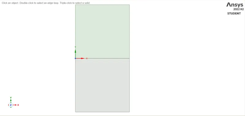
iii. Steps to Generate the Surfaces: -

SpaceClaim `->` Select "Return to 3D Mode" from Graphic Window

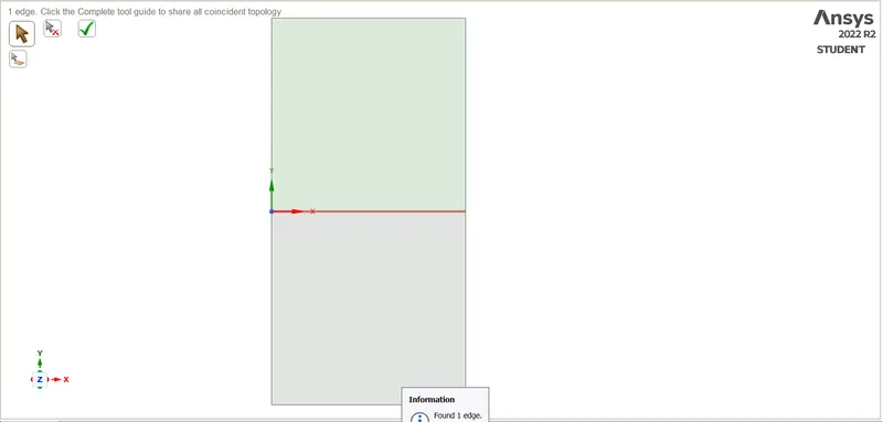
iv. Steps to Share Topology between the Solid and Fluid: -

SpaceClaim `->` Workbench `->` `ubrace("Share")_("It will auto-detect the Common Boundaries")` `->` Enter

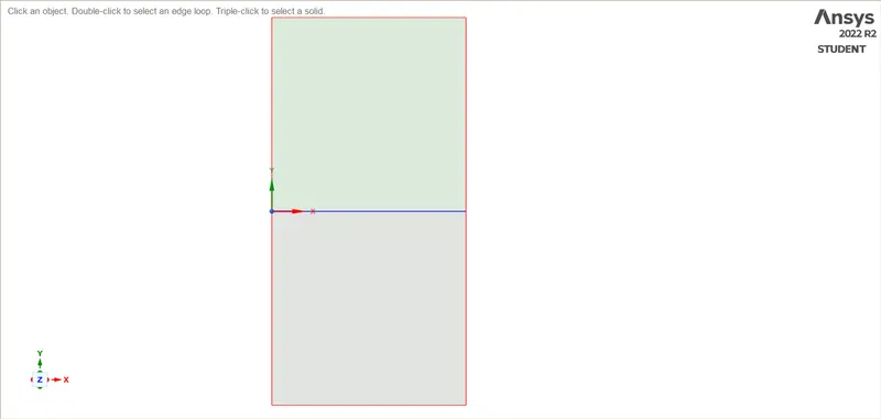Common Edge Between both Surfaces	Shared Common Edge

C. Opening Mechanical(Meshing) and Meshing the Geometry: -

i. Steps to Open Meshing: -

Ansys Workbench `->` Project Schematic `->` Project `->` Mesh `->` Right-Click `->` Edit

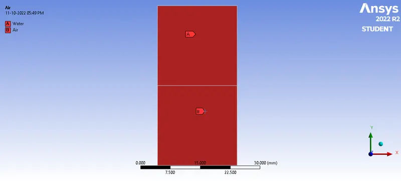
ii. Steps to Name the Boundary: -

Mechanical(Meshing) `->` Model Working Window `->` Select the Boundary `->` Click N `->` Give the desired Name `->` Enter

iii. Steps to Create the Mesh: -

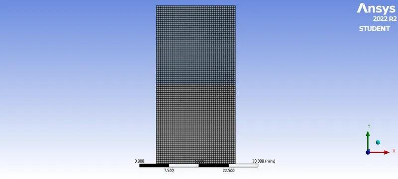
Outline Window `->` Select Mesh `->` Details of Mesh Window `->` Defaults `->` Element Size is set to the desired Value

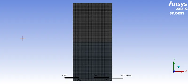Mesh generated with a base size = 0.5mm	Mesh generated with a base size = 0.2mm

D. Setuping the Physics and Boundary Conditions: -

i. Steps to Open Ansys Fluent: -

Ansys Workbench `->` Project Schematic `->` Project `->` Setup `->` Right-Click `->` Edit

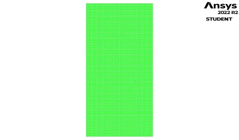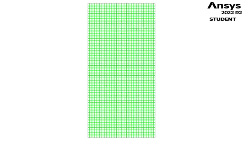
Mesh with base size = 0.5mm in Fluent	Mesh with base size = 0.2mm in Fluent

ii. Steps to Check Mesh: -

Fluent `->` Outline View Window `->` Setup `->` General `->` Mesh `->` Check

iii. Steps to Set up the Physics: -

a. Setting Viscous Solver: Fluent `->` Physics `->` Models `->` Viscous `->` `ubrace("Select Desired Viscous Model")_("In our case Select Laminar")`

b. Setting/Creating Material: Fluent `->` Physics `->` Materials `->` Create/Edit... `->` Select/Create the desired Fluid `->` Enter

c. Setting Multiphase: Fluent `->` Physics `->` Models `->` Multiphase `->` Model `->` `ubrace("Select Desired MultiPhase Model")_("In our case Select Volume of Fluid Method")` `->` Select "Implicit" under Formulation `->` Apply

d. Setting Primary and Secondary Phases: Fluent `->` Physics `->` Models `->` Multiphase `->` Phases `->` Set Desired Primary and Secondary Phases `->` Apply

iv. Steps to Initialize and Set Desired Graphical Views: -

a. Initializing: Fluent `->` Solution `->` Initialization `->` Initialize

b. Patch the Materials: Fluent `->` Solution `->` Patch `->` Select "Water" in Phases `->` Volume Fraction `->` Set Water Value as 1 `->` Patch `->` Air/User Defined Fluid as 0 `->` Patch

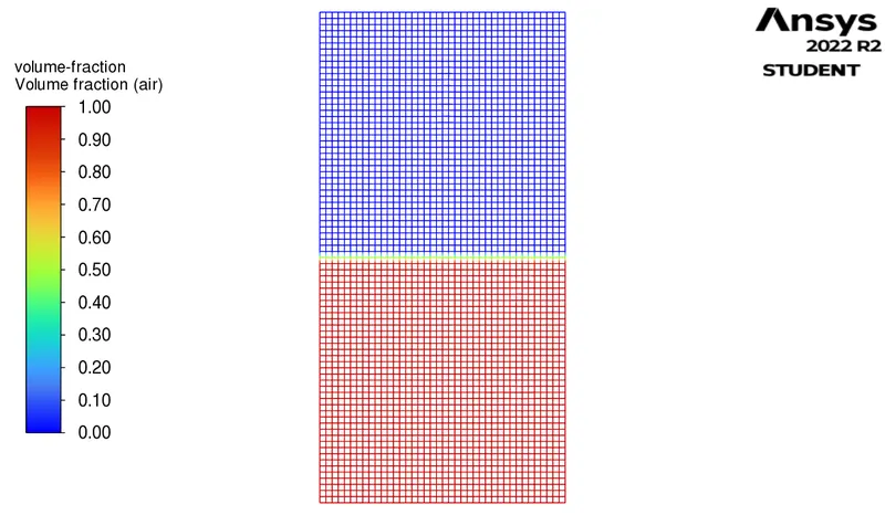
c. Setting the desired Contour: Fluent `->` Results `->` Graphics `->` Contours `->` New `->` Rename `->` Select Variable for Contour of `->` Select Surface `->` Save/Display

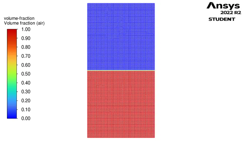Volume Fraction of Air at t = 0 for base Mesh = 0.5mm	Volume Fraction of Air at t = 0 for base Mesh = 0.2mm

Steps to Analyse the Conjugate Heat Transfer Analysis of Exhaust Port: -

A. Performing Calculations and Developing Results: -

i. Steps to Open Fluent: -

Ansys Workbench `->` Project Schematic `->` Project `->` Setup `->` Right-Click `->` Edit

ii. Steps to Run Calculations: -

a. Setting up Time Step Size: Fluent `->` Solution `->` Run Calculations `->` `ubrace("Setting Desired Iterations in Time Step Size")_("In Our Case Time Step Size was set to 0.002")`

b. Setting up Time Step: Fluent `->` Solution `->` Run Calculations `->` Setting Desired Time Step Size

c. Running Calculations: Fluent `->` Solution `->` Run Calculations `->` Calculate

Simulation Animation: -

A. For Course Mesh For Air and Water: -

B. For Fine Mesh For Air and Water: -

C. For Fine Mesh For User Defined Fluid and Water: -

Observations and Reasons: -

A. Comparision Between Course and Fine Mesh: -

Course Mesh(base Size = 0.5mm) Fine Mesh(base Size = 0.2mm)

The following are the observations that can be made: -

i. The Expansion Rate of the Bubble of Air in both Mesh Sizes is the same.

ii. After the Instability when the mixture becomes turbulent the course mesh is unable to demonstrate the turbulence.

iii. The Viscous effect near the Walls is better Estimated in the Fine Mesh size than in the Course Mesh size.

iv. The small eddies are not estimated correctly in the Course Mesh

The Reasons for these differences are as follows: -

i. As the Volume of Fraction Method is used each Mesh is estimating the amount of Phase 1 and Phase 2 present in them due to which in the course mesh size the Average values are estimated compared to Fine Mesh.

ii. As in the Fine Mesh the Size of the grids near the Walls are very fine due to which the no-slip condition is estimated correctly.

B. Difference between Air & Water and User Defined Fluid & Water: -

As the Density of Air is far less compared to Water than that of User Defined Fluid and Water the rate of Bubble expansion within the Air and Water is faster Compared to User Defined Fluid and Water. This expansion can also be estimated using the dimensionless number Atwood Number. The higher the Atwood Number the higher the expansion of bubbles.

The expansion rate can also be estimated using the Formula(For Inviscid Condition)

Penetration distance(d) = (Atwood Number)x(Net gravitational Acceleration)x(`time^2`)

The Above Mentioned Formula gives the results for Inviscid fluids but still can be used to estimate the difference of the Penetration distance within the same time or Penetration Time for the same distance.

Now,

Atwood Number of User-Defined Fluid and Water `<` Atwood Number of Air and Water

`=>` Rate of Bubble expansion in User-Defined Fluid and Water `<` Rate of Bubble expansion in Air and Water