Week 5 - Rayleigh Taylor Instability

Aim:- To simulate the Rayleigh Taylor instability for 2 fluids.

Objective:-

1. What are some practical CFD models that have been based on the mathematical analysis of Rayleigh Taylor waves? In your own words, explain how these mathematical models have been adapted for CFD calculations.
2. Perform the Rayleigh Taylor instability simulation for 2 different mesh sizes with the base mesh being 0.5 mm. Compare the results by showing the animations( Attach them from your google drive). Observe the differences in the animation and explain the effect of mesh size on simulation. Also, explain why a steady-state approach might not be suitable for these types of simulation.[ Choose Air and Water for this simulation]
3. Run one more simulation with water and user-defined material(density = 400 kg/m³, viscosity = 0.001 kg/m-s) for refined mesh.
4. Define the Atwood Number. Find out the Atwood number for both the cases and explain how the variation in Atwood number in the above two cases affects the behavior of the instability.

Theory:-

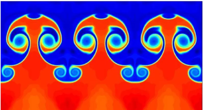
RT instability is the instability of an interface between two fluids of different densities which occurs when the lighter fluid is pushing the heavier fluid. Water suspended atop oil is an everyday example of Rayleigh–Taylor instability, and it may be modeled by two completely plane-parallel layers of immiscible fluid, the more dense on top of the less dense one and both subject to the Earth's gravity. The equilibrium here is unstable to any perturbations or disturbances of the interface: if a parcel of heavier fluid is displaced downward with an equal volume of lighter fluid displaced upwards, the potential energy of the configuration is lower than the initial state. Thus the disturbance will grow and lead to a further release of potential energy, as the more dense material moves down under the (effective) gravitational field, and the less dense material is further displaced upwards.

Practical CFD models that have been based on mathematical analysis of RT waves...

1. Kelvin-Helmholtz instability
2. Richtmyer-Meshkov instability
3. Plateau-Rayleigh instability

Kelvin-Helmholtz instability- This instability typically occurs when there is velocity shear in a single continuous fluid, or additionally where there is a velocity difference across the interface between two fluids. A common example is seen when wind blows across a water surface; the instability constant is able to manifest itself through waves on water surface. The Kelvin-Helmholtz instability is not only restricted to a water surface as clouds, but is evident through other natural phenomena as ocean and the sun's corona.

Richtmyer-Meshkov instability- This occurs when two fluids of different density are impulsively accelerated. Normally this is by the passage of a shock wave. The development of the instability begins with small amplitude perturbations which initially grow linearly with time. This is followed by a nonlinear regime with bubbles appearing in the case of a light fluid penetrating a heavy fluid, and with spikes appearing in the case of a heavy fluid penetrating a light fluid. A chaotic regime eventually is reached and the two fluids mix. This instability can be considered the impulsive-acceleration limit of the Rayleigh Taylor instability.

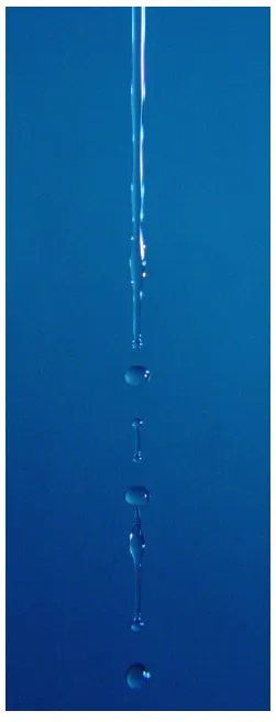
Plateau-Rayleigh instability- This instability, often just called the Rayleigh instability, explains why and how a falling stream of fluid breaks up into smaller packets with the same volume but less surface area. It is related to the RTI and is part of a greater branch of fluid dynamics concerned with fluid thread breakup. This fluid instability is exploited in the design of a particular type of ink jet technology whereby a jet of liquid is perturbed into a steady stream of droplets. The driving force of the Plateau–Rayleigh instability is that liquids, by virtue of their surface tension, tend to minimize their surface area.

CFD:-Computational fluid dynamics or CFD is the analysis of systems involving fluid flow, heat transfer and associated phenomena such as chemical reactions by means of computer-based simulation.

Practical application in current scenario

• aerodynamics of aircraft and vehicles: lift and drag
  • hydrodynamics of ships
  • power plant: combustion in internal combustion engines and gas
  turbines
  • turbomachinery: flows inside rotating passages, diffusers etc.
  • electrical and electronic engineering: cooling of equipment including
  microcircuits
  • chemical process engineering: mixing and separation, polymer moulding
  • external and internal environment of buildings: wind loading and
  heating/ventilation
  • marine engineering: loads on off-shore structures
  • environmental engineering: distribution of pollutants and effluents
  • hydrology and oceanography: flows in rivers, estuaries, oceans
  • meteorology: weather prediction
  • biomedical engineering: blood flows through arteries and veins

CFD Work Flow:- CFD codes are structured around the numerical algorithms that can tackle fluid flow problems. In order to provide easy access to their solving power all commercial CFD packages include sophisticated user interfaces to input problem parameters and to examine the results

Its threee step process
(i) a pre-processor

involves defination of geometry, grid generation, selection of phenomenon that need to model

(ii) a solver

intergration of governing equation, discretisation and solution

(iii) a post-processor

ploting of contour, graphs and making movies.

In solving fluid flow problems we need to be aware that the underlyingphysics is complex and the results generated by a CFD code are at best asgood as the physics (and chemistry) embedded in it and at worst as good asits operator with CFD

Solving and Modeling Approch:-

There are no way present to understand and analyse the effeciveness of the mixiing tee model.

1. analytical approch

2. simulation approch

3. experimental approch

using analytical approch and experimental approch is time consuming and high cost senario. this could be eliminated by using simulation approch in which we can analyse the system with the actual codition we are intrested in.

To do this we are using ansys fluent solver

we are using fluid flow analysis using Fluent solver because we are interested in the total effectiveness of the fluid in the mechnical tee model, here we are using two different models to analyse the effectiveness of the mixing of fluid.

Approch we are using.

1. We need to open Ansys workbench

2. Choose the Appropiate Solver

3. Assign Appropiate name

4. Choose geometry and select new spaceclaim model.

5. Load the appropiate file

6. Implement the geometrical operation

7. Apply the mesh and provide name selection

8. Choose setup, select the appropiate model

9. Initalisation and running the simulation

10. Result making i.e. countour plots graphs

1. Opening Ansys workbench

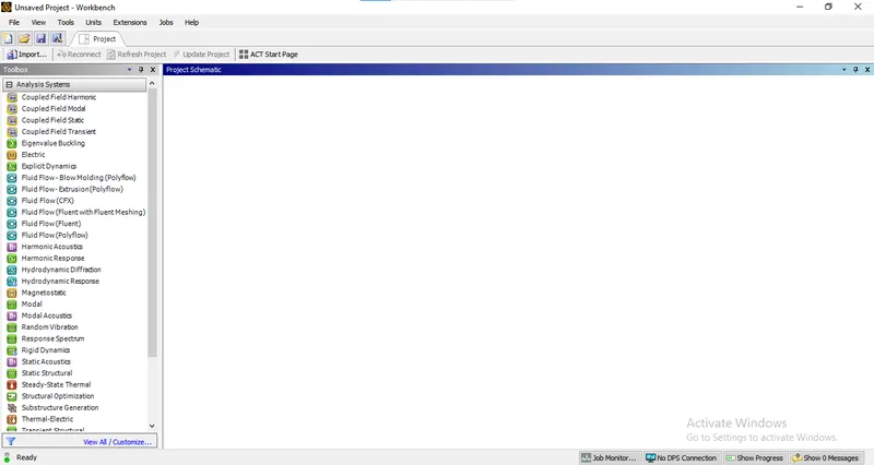
2. Choose the Appropiate Solver

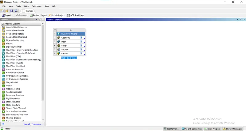
3. Assign Appropiate name:- Instability

4. Opening of space claim geometry do to geometrical operation

by using the sketch mode in space claim we create a simple geometry to analyse the rayleih instabliy, to simulate this we create two different rectangles with 20mm*20mm we need to use design>add new component

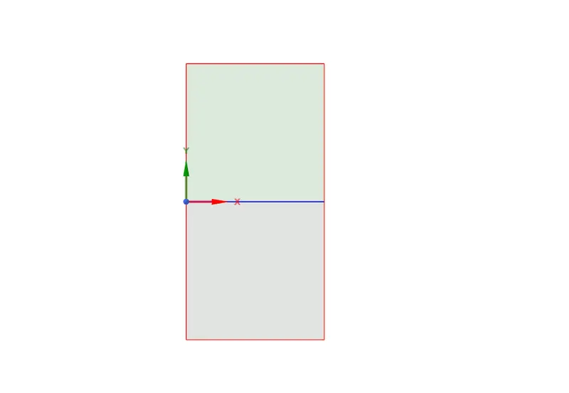
Draw 1st rectangle> move to 3d mode

add new component

draw 2nd rectangle>move to 3d mode

use share topology

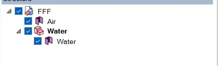
we done with geometry parts. Now we can start with meshing.

Meshing

now we can starting meshing with mesh length as 5mm

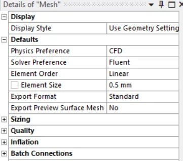
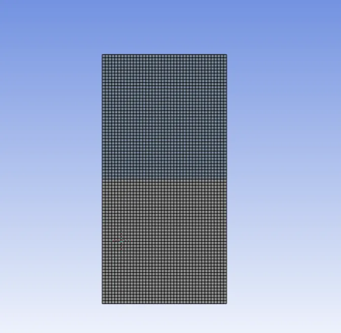
We done with mesh part.

Setup

Settings

Solver	Transient State
Energy Equation	Off
Model	Laminar
Inlet	Inlet
Outlet	Pressure Outlet
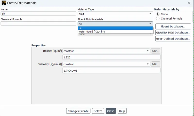
Material_(Fluid)	Air(user defined), Water
Cell Zone Condition	Air, Water
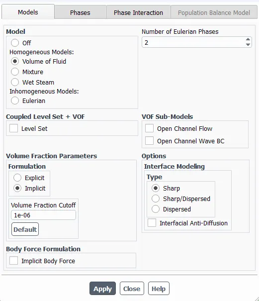
Multiface	VOF

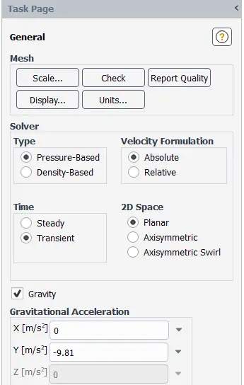
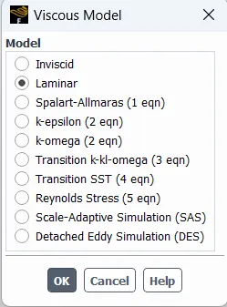
Add materials

Go to Multiface. Enable VOF

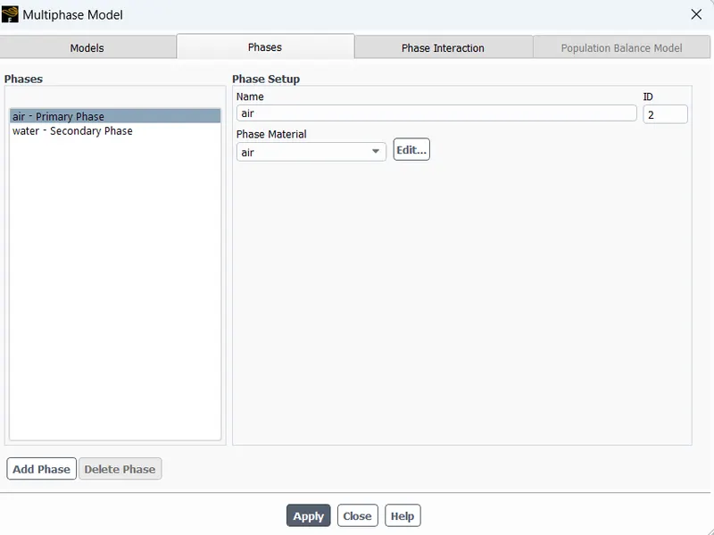
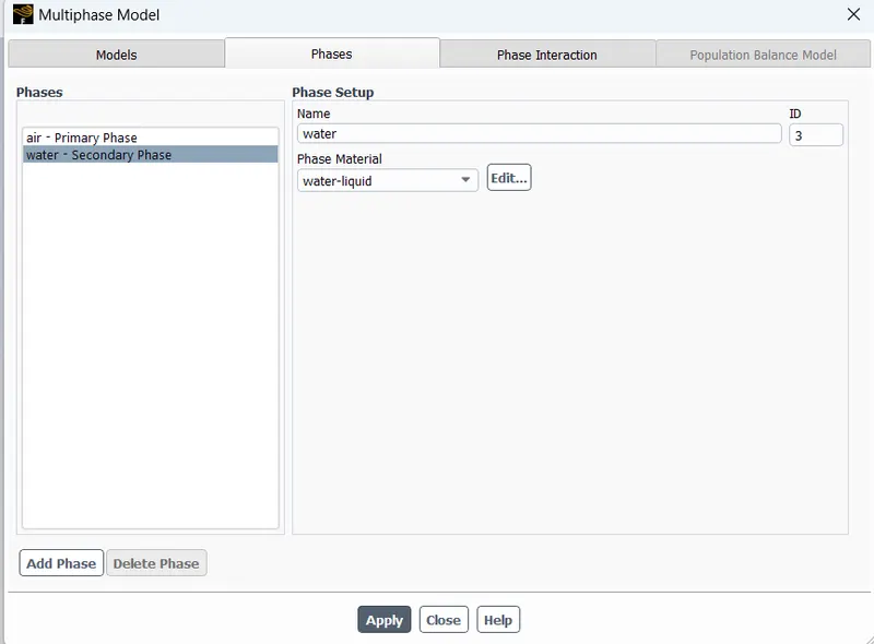
Now we intialise the setup.

Patch the volume fraction.

patching

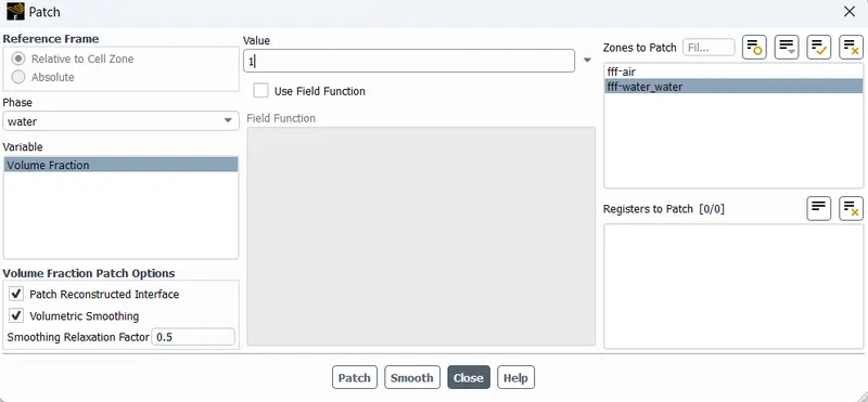
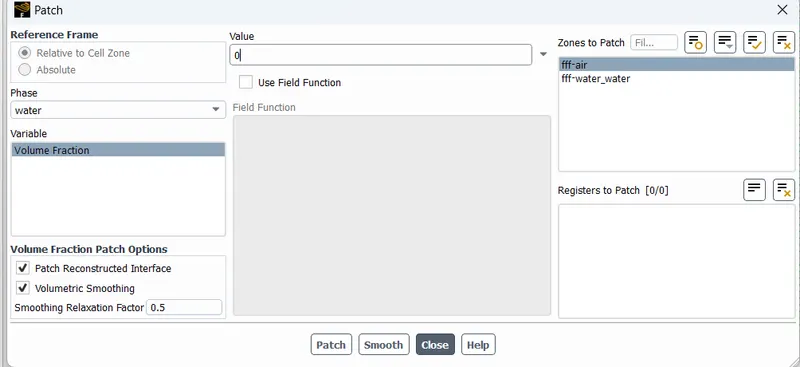
patching>choose phase as water>choose variable>select the zone to patch>enter the vale >click patch

For water phase use 1

for liquid use 0

Now we can create the contour for phase.

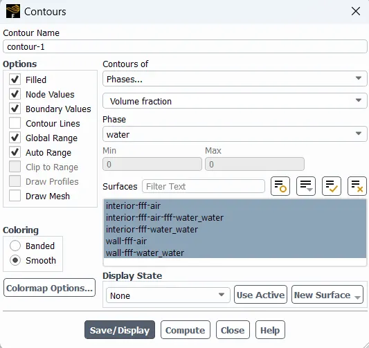
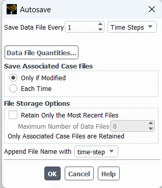
now we use autosave option to save the simulation data we will save for each iteration.

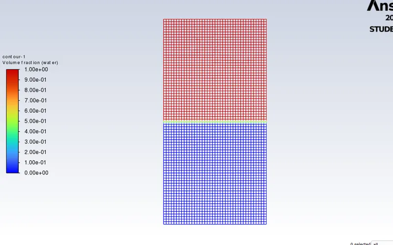
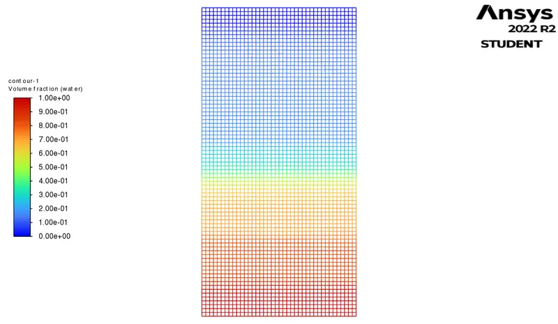
Initial Condition

Result:-

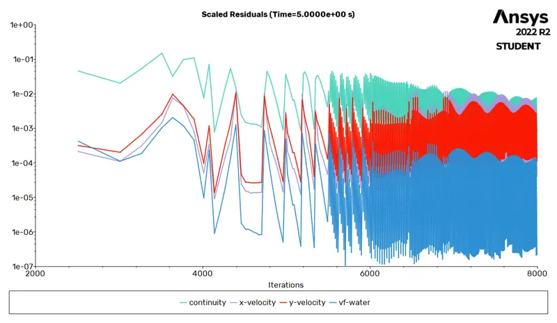
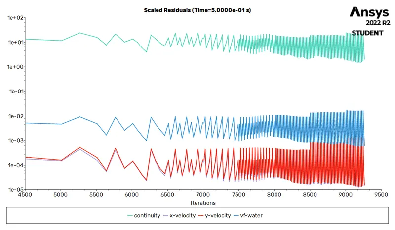
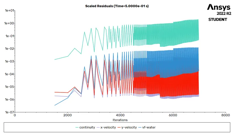
1. Residuals

Mesh Length as .5 mm Material Air, Water	Mesh Length as .1 mm Material Air, Water	Mesh Length as .1 mm Material Water, User Defined

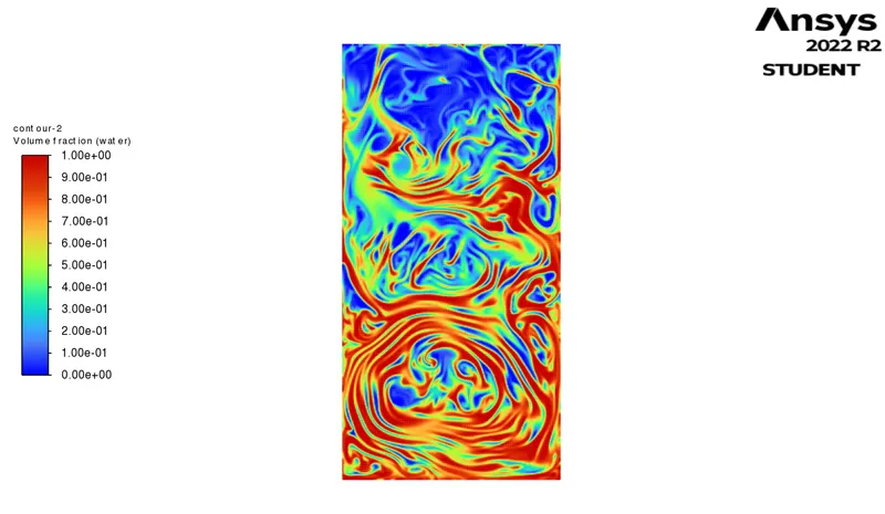
2. Volume Contour

Mesh Length as .5 mm Material Air, Water	Mesh Length as .1 mm Material Air, Water	Mesh Length as .1 mm Material Water, User Defined

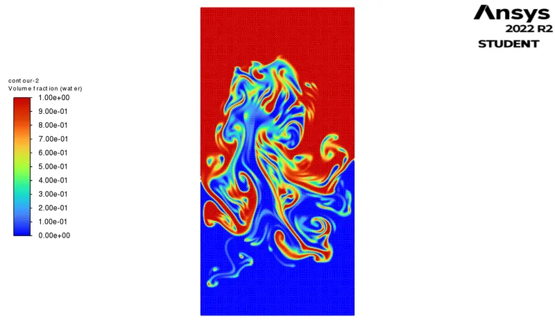3. Video Links

1. Mesh Length as .5 mm, Material Air, Water

https://drive.google.com/file/d/104l0K81wuQ-tT2oIh_YNY-W2qoDvnlGH/view?usp=sharing

2. Mesh Length as . 1mm, Material Air, Water

https://drive.google.com/file/d/1mcGXr7X7jQW3sARdi8Rpfx2rWYb5U5w2/view?usp=sharing

3. Mesh Length as .1 mm, Material Air, User Defined

https://drive.google.com/file/d/1-qFBn_aOQYQHLdVDwvsu6Lz8DRhgDXCv/view?usp=sharing

Atwood Number It is a dimensionless number that is used to study hydrodynamic instabilities in density stratified flows.

A = rho1- rho2/rho1+rho2

where

rho1 is density of heavier fluid

rho2 is density of lighter fluid

For Air-water RT instability,

rho1 = 998.2 kg/m^3 [Water density]

rho2= 1.225 kg/m^3 [Air density]

A = (998.2-1.225)/(998.2+1.225)

A = .998

For Water-user defined RT instability

rho1= 988.2 kg/m^3[Water density]

rho2 = 400 kg/m^3 [Air density]

A = (998.2-400)/(998.2+400)

A = .423

Inference

1. finer the mesh excat will be the result.

2. finer mesh iincreases computational time

3. instablity are changing in unpredictable manner as a function of time.

4. smaller the mesh size higher the time taken by the heavy fluid to settle.

5. as the atwood no lowes chance of bubbles and spike formation increases